
In his April 1 post, Paul Allison pointed out several attractive properties of the logistic regression model. But he neglected to consider the merits of an older and simpler approach: just doing linear regression with a 1-0 dependent variable. In both the social and health sciences, students are almost universally taught that when the outcome variable in a regression is dichotomous, they should use logistic instead of linear regression. Yet economists, though certainly aware of logistic regression, often use a linear model to model dichotomous outcomes.
Which probability model is better, the linear or the logistic? It depends. While there are situations where the linear model is clearly problematic, there are many common situations where the linear model is just fine, and even has advantages.
LEARN MORE IN ONE OF OUR SHORT SEMINARS
Interpretability
Let’s start by comparing the two models explicitly. If the outcome Y is a dichotomy with values 1 and 0, define p = E(Y|X), which is just the probability that Y is 1, given some value of the regressors X. Then the linear and logistic probability models are:
p = a0 + a1X1 + a2X2 + … + akXk (linear)
ln[p/(1-p)] = b0 + b1X1 + b2X2 + … + bkXk (logistic)
The linear model assumes that the probability p is a linear function of the regressors, while the logistic model assumes that the natural log of the odds p/(1-p) is a linear function of the regressors.
The major advantage of the linear model is its interpretability. In the linear model, if a1 is (say) .05, that means that a one-unit increase in X1 is associated with a 5 percentage point increase in the probability that Y is 1. Just about everyone has some understanding of what it would mean to increase by 5 percentage points their probability of, say, voting, or dying, or becoming obese.
The logistic model is less interpretable. In the logistic model, if b1 is .05, that means that a one-unit increase in X1 is associated with a .05 increase in the log odds that Y is 1. And what does that mean? I’ve never met anyone with any intuition for log odds.
How intuitive are odds ratios?
Because the log odds scale is so hard to interpret, it is common to report logistic regression results as odds ratios. To do this, we exponentiate both sides of the logistic regression equation and obtain a new equation that looks like this:
p/(1-p) = d0 × (d1)X1 × (d2)X2 × … × (dk)Xk
On the left side we have the odds and on the right side we have a product involving the odds ratios d1 = exp(b1), d2 = exp(b2), etc.
Odds ratios seem like they should be intuitive. If d1 = 2, for example, that means that a one-unit increase in X1 doubles the odds that Y is 1. That sounds like something we should understand.
But we don’t understand, really. We think we understand odds because in everyday speech we use the word “odds” in a vague and informal way. Journalists commonly use “odds” interchangeably with a variety of other words, such as “chance,” “risk,” “probability,” and “likelihood”—and academics are often just as sloppy when interpreting results. But in statistics these words aren’t synonyms. The word odds has a very specific meaning—p/(1-p)—and so does the odds ratio.
Still think you have an intuition for odds ratios? Let me ask you a question. Suppose a get-out-the-vote campaign can double your odds of voting. If your probability of voting was 40% before the campaign, what is it after? 80%? No, it’s 57%.
If you got that wrong, don’t feel bad. You’ve got a lot of company. And if you got it right, I bet you had to do some mental arithmetic[1], or even use a calculator, before answering. The need for arithmetic should tell you that odds ratios aren’t intuitive.
Here’s a table that shows what doubling the odds does to various initial probabilities:
|
Before doubling |
After doubling | ||
|
Probability |
Odds |
Odds |
Probability |
|
10% |
0.11 |
0.22 |
18% |
|
20% |
0.25 |
0.50 |
33% |
|
30% |
0.43 |
0.86 |
46% |
|
40% |
0.67 |
1.33 |
57% |
|
50% |
1.00 |
2.00 |
67% |
|
60% |
1.50 |
3.00 |
75% |
|
70% |
2.33 |
4.67 |
82% |
|
80% |
4.00 |
8.00 |
89% |
|
90% |
9.00 |
18.0 |
95% |
It isn’t simple. The closest I’ve come to developing an intuition for odds ratios is this: If p is close to 0, then doubling the odds is approximately the same as doubling p. If p is close to 1, then doubling the odds is approximately the same as halving 1-p. But if p is in the middle—not too close to 0 or 1—then I don’t really have much intuition and have to resort to arithmetic.
That’s why I’m not crazy about odds ratios.
How nonlinear is the logistic model?
The logistic model is unavoidable if it fits the data much better than the linear model. And sometimes it does. But in many situations the linear model fits just as well, or almost as well, as the logistic model. In fact, in many situations, the linear and logistic model give results that are practically indistinguishable except that the logistic estimates are harder to interpret (Hellevik 2007).
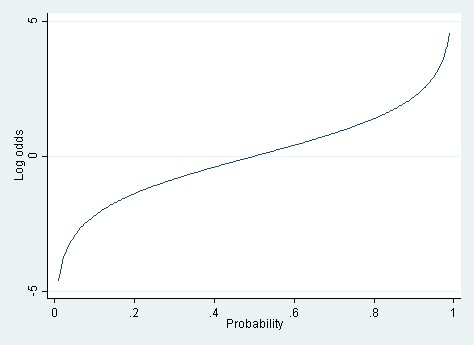
For the logistic model to fit better than the linear model, it must be the case that the log odds are a linear function of X, but the probability is not. And for that to be true, the relationship between the probability and the log odds must itself be nonlinear. But how nonlinear is the relationship between probability and log odds? If the probability is between .20 and .80, then the log odds are almost a linear function of the probability (cf. Long 1997).
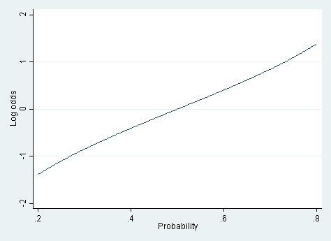
It’s only when you have a really wide range of probabilities—say .01 to .99—that the linear approximation totally breaks down.
When the true probabilities are extreme, the linear model can also yield predicted probabilities that are greater than 1 or less than 0. Those out-of-bounds predicted probabilities are the Achilles heel of the linear model.
A rule of thumb
These considerations suggest a rule of thumb. If the probabilities that you’re modeling are extreme—close to 0 or 1—then you probably have to use logistic regression. But if the probabilities are more moderate—say between .20 and .80, or a little beyond—then the linear and logistic models fit about equally well, and the linear model should be favored for its ease of interpretation.
Both situations occur with some frequency. If you’re modeling the probability of voting, or of being overweight, then nearly all the modeled probabilities will be between .20 and .80, and a linear probability model should fit nicely and offer a straightforward interpretation. On the other hand, if you’re modeling the probability that a bank transaction is fraudulent—as I used to do—then the modeled probabilities typically range between .000001 and .20. In that situation, the linear model just isn’t viable, and you have to use a logistic model or another nonlinear model (such as a neural net).
Keep in mind that the logistic model has problems of its own when probabilities get extreme. The log odds ln[p/(1-p)] are undefined when p is equal to 0 or 1. When p gets close to 0 or 1 logistic regression can suffer from complete separation, quasi-complete separation, and rare events bias (King & Zeng, 2001). These problems are less likely to occur in large samples, but they occur frequently in small ones. Users should be aware of available remedies. See Paul Allison’s post on this topic.
Computation and estimation
Interpretability is not the only advantage of the linear probability model. Another advantage is computing speed. Fitting a logistic model is inherently slower because the model is fit by an iterative process of maximum likelihood. The slowness of logistic regression isn’t noticeable if you are fitting a simple model to a small or moderate-sized dataset. But if you are fitting a very complicated model or a very large data set, logistic regression can be frustratingly slow.[2]
The linear probability model is fast by comparison because it can be estimated noniteratively using ordinary least squares (OLS). OLS ignores the fact that the linear probability model is heteroskedastic with residual variance p(1-p), but the heteroscedasticity is minor if p is between .20 and .80, which is the situation where I recommend using the linear probability model at all. OLS estimates can be improved by using heteroscedasticity-consistent standard errors or weighted least squares. In my experience these improvements make little difference, but they are quick and reassuring.
Paul von Hippel is an Associate Professor in the LBJ School of Public Affairs at the University of Texas, Austin, with affiliations and courtesy appointments in Sociology, Population Research, and Statistics and Data Science.
References
Hellevik, O. (2007) Linear versus logistic regression when the dependent variable is a dichotomy. Quality & Quantity, 43(1), 59–74. http://doi.org/10.1007/s11135-007-9077-3
King, G., & Zeng, L. (2001) Logistic Regression in Rare Events Data. Political Analysis, 9(2), 137–163. http://doi.org/10.2307/25791637
Long, J. S. (1997) Regression Models for Categorical and Limited Dependent Variables (1st ed.). Sage Publications, Inc.
[1] Here’s the mental arithmetic that I did. A probability of 40% is equivalent to odds of 2/3. Doubling those odds gives odds of 4/3. And odds of 4/3 are equivalent to a probability of 4/7, which in my head I figured was about 56%. When I wrote this footnote, though, I checked my mental arithmetic using Excel, which showed me that 4/7 is 57%.
[2] In current work, my colleagues and I are using a hierarchical, spatially correlated model to estimate the probability of obesity among 376,576 adults in approximately 2,400 US counties. The computational methods are demanding, and switching from a logistic to a linear probability model reduced our runtime from days to less than an hour.
Comments
You mentioned that odds-ratios are less intuitive than we may believe. What you said about misunderstanding the implications of doubling the odds-ratio makes a lot of sense. However, I have always understood that the value of the odds ratio itself can give us information about the differences in the probability of an outcome conditional on a particular property. Take for example running a logistic regression where the dependent variable is whether someone falls ill or not (0= does not fall ill and 1= falls ill) and one of the explanatory variables is gender (with 0 coded for females and 1 coded for males). If the output in terms of odds ratios is 2 for the gender variable, I have understood this to mean that a male is twice as likely to fall ill compared to a female (ie, the probability of the male falling ill is double that of the female). Is this an incorrect interpretation?
If the 2 here means that it is the odds ratio that has doubled and not the probability, what is the initial reference point that it is doubling from?
No, an odds ratio of 2 does not mean that the probability is twice is large for a male as for a female. That would be a relative risk ratio. Suppose the probability of a female falling ill is .50. The odds of her falling ill is then 1. Doubling that would give an odds of 2, which translates into a probability of .667.
Great thanks for a very clear and informative article! I would very much like to hear your comments on an article that seems to agree with your position, making a strong case for the Linear Probablity Model under certain conditions. But the article goes further showing that there are great problems with logistic models for a number of standard situations. But before writing a new mail to you, I would just like to know if you still read and answer questions since your article was from 2015 and there were no dates in the questions and comments. Best wishes Dan
Hi, I’m replying for Paul von Hippel. Can you give us a reference for the article? And you may want to take a look at my latest blog post on predicted probabilities for LPMs: https://statisticalhorizons.com/better-predicted-probabilities/
I have questions about what constitutes “better.” The linear model can be estimated in Excel, an advantage. While the linear model can have predicted values outside the 0-1 range, what happens if you just assign a value of 1 to a prediction of 1.1 and 0 to a prediction of -0.2. If we just care about the 0-1 prediction, how well do the models compare? For logit, a prediction of 0.6 is assigned 1. Have any studies compared prediction accuracy? Because the linear model is mis-specified, what problems does this present for confidence intervals and hypothesis testing?
The dependant variable assume value either 0 or 1. So in order to fit linear regression how do you calculate p = E(Y/X) for each record? Also here do we use OLS estimator or MLE?
p is just Xb. Only problem is p could be greater than 1 or less than 0. It would be possible to do MLE but it will fail if Xb is out of bounds.
A student just pointed this article out to me.
I am rather surprised that computational aspects are even a question today, and that there is an effort to justify a model that is clearly inappropriate for this situation in so many ways.
If there is any interest in using the model for prediction and accounting for the uncertainty in the prediction then I simply dont see how an adherent of the LPM would make a case for its utility
If there is a somewhat naive interest in identifying regression coefficients – and talking about the linear effect of a predictor on the probability of the outcome then perhaps you could make an argument, but certianly the confidence intervals of the coefficient would not be proper and hence you would not be able to say anything useful
FInally, the idea that the model is ok if the predicted p is between 0.2 and 0.8 seems rather ridiculous.
A) so you suggest one uses the model in all cases when the output is in this range and reject it in others? potentially the cases where p is outside this range are the ones of greatest interest from a risk perspective
B) these thresholds seem arbitrary, and again neglect a consideration of sample size or uncertainty associated with the prediction
I am sorry to be so negative, but posts such as this do create confusion for students and hence bear discussion
Readers may also be interested in this article by Cheung (2007):
https://www.ncbi.nlm.nih.gov/pubmed/18000021
Cheers,
Bruce
Thank you for writing this clear and helpful post. I am sure to return to it and reference it.
I wonder if you would comment on the comparison between the two models when one wishes to include fixed effects. The LPM certainly retains the computational advantage in the FE case. I think it retains the interpretability advantage too—but I would really appreciate hearing your take on that, as well as whether the same rule of thumb re: moderate probabilities applies.
I haven’t come across a discussion of how the two models compare when FE are included elsewhere, but if you know of sources I ought to be consulting, I’d appreciate you pointing me toward anything else. Thanks again!
This is an interesting article, and I think anybody using statistical models should realise that “all models are wrong” and not feel constrained by conventions. It will certainly make me consider the LPM in future.
However, I have a bit of a problem with the advice that if p is between 0.2 and 0.8 it’s fine to use LPM. You are talking about the probability, conditional on the covariates, but the whole point of regression is that usually we don’t know the probability, conditioning on the covariates, before we run the model. p-hat is an output of the model.
Especially when we have lots of covariates and some are continuous, it is impossible to say whether there are some regions of the design space where p-hat is closer to 1 or 0, and probably very likely that there will be.
I haven’t looked into this properly, but I suspect that a LPM is much more sensitive to high-leverage points at the extremes of covariate values.
Even more problematically, extreme covariate values will bias the coefficient downwards (attenuation), whether or not the corresponding outcome is 1 or 0, because the LPM expects outcomes that become large in absolute value as covariates become large in absolute value.
For example, if you have a mean centred, standardised covariate, and the corresponding intercept and coefficient are 0.5 and 0.2, then you add a data point at X=4, this data point will bias the slope down, whether or not it is a 1 or 0, because the model expects 1.3.
I don’t think this concern is abstract because with lots of covariates you’re bound to have some high-leverage points.
You mention the rare event bias — I have reason to suspect this bias is mythical — perhaps you can comment: http://stats.stackexchange.com/questions/169199/rare-event-logistic-regression-bias-how-to-simulate-the-underestimated-ps-with
I’m not sure I understand your simulation. You’re simulating samples of a Bernoulli variable Y with n=100 and p=.01. If you do this, then 37% of your simulated samples will have Y=0 in all 100 observations. What do you do then? Since the log of 0 is undefined, you can’t run logistic regression on those datasets using maximum likelihood. You have to use an estimator that smooths the estimated probability away from zero.
This is one of the problems that the logistic model has near p=0. By the way, in this situation the linear probability model is unbiased.
Great point, and see updates to my link as a result. R failed to throw a warning because its “positive convergence tolerance” actually gets satisfied. More liberally speaking, the MLE exists and is minus infinity, which corresponds to p=0, so my new approach is to just use p = 0 in the edge case. The only other coherent thing I can think of doing is discarding those runs of the simulation where y is identically zero, but that would clearly lead to results even more counter to the initial King & Zeng claim that “estimated event probabilities are too small!
When all the Ys are 0, it’s reasonable to estimate p as 0. But that’s not an estimate that comes from a logistic regression model. So you can’t use it to claim that logistic regression maximum likelihood estimates are unbiased when p is near 0.
Let’s go back to the previous situation, where you were throwing out datasets if all the Ys were 0. Among the datasets that remain, the expectation of Y isn’t .01 any more. It’s about .0158. If the estimand is .0158, and your estimates average .01, then you have bias.
That sounds good. So, ultimately I wonder if you would interpret your latter conclusion to mean that King & Zheng’s claim that “estimated event probabilities are too small” is incorrect.
I replicated your simulation, using SAS PROC LOGISTIC. I simulated n=100 observations on a variable Y drawn from a Bernouilli distribution with p=.01, and then fit an intercept-only logistic model to estimate P(Y=1) with no correction for rare-events bias. I replicated this simulation 10,000 times.
Here is what I found:
(1) Across all the datasets, 1% of cases had Y=1.
(2) In 36% of the datasets, no cases had Y=1, so I could not run the logistic regression.
(3) In the remaining 64% of datasets, 1.57% of cases had Y=1 and I could run the logistic regression.
(4) Across those datasets, the average predicted probability from the logistic regression was 1.57%.
So you’re right: there’s no bias in these predicted probabilities. The predicted probability is equal to the true probability.
This is true not just on average, but within each simulated dataset. If there’s one case with Y=1, then the logistic regression will give a predicted probability of .01. If there are two cases with Y=2, the predicted probability will be .02. Etc.
However, this does not contradict King and Zeng’s results. If you look at their equation (16), you’ll see that the bias is a function of the regressors X, and there are no Xs in this simulation. Similarly, King & Zeng’s Figure 7 shows that there is essentially no bias when X=0.
You might consider seeing if you can replicate King & Zeng’s simulation.
You noted that “The log odds ln[p/(1-p)] are undefined when p is equal to 0 or 1.” This infinity problem in doing OLS on Log Odds is normally avoided by grouping individual data points, but choosing these groups is somewhat arbitrary. An alternate approach is to replace p=0 with p=epsilon and to replace p=1 with p=1-epsilon where epsilon is small (say 0.001). This avoids the infinity problem and the grouping problem. The OLS solution for Log Odds is qualitatively close to the MLE solution. The theoretical defects in this alternate approach are obvious, but pedagogically it allows beginning students using Excel to deal with binary outcomes. Q. What do you think of this alternate OLS Ln Odds approach?
I’m not sure how you’re replacing p=0 with p=epsilon? What some people do is add a row to the data containing a “pseudo-case” where Y=1 and the X values are typical for cases with Y=0. Then they run logistic regression as usual, perhaps assigning a low weight to the pseudo-case.
The approach is ad hoc and it involves some arbitrary choices. How many pseudo-cases do you need? What weight should you assign them? Still, it’s easy, it runs quickly, and the estimates can be serviceable.
There are more principled approaches when p is close to 0 or 1, though. See Paul Allison’s post on logistic regression for rare events:
https://statisticalhorizons.com/logistic-regression-for-rare-events/
When every observation is either 0 or 1, I don’t think this is an acceptable approach. Your coefficients will depend too heavily on the choice of epsilon.
It depends on whether you intend your conclusions to apply to your study sample, or to the US population. If you’re only generalizing to the study sample, then the probability of the disease is 50%, and — provided there are no covariate values for which the probability is more than 80% or less than 20% — you can safely use a linear probability model.
On the other hand, if you want to generalize to the US population, then you need to apply sample weights so that the weighted proportions in your sample estimate the corresponding proportions in the population. Since the weighted probability of disease in the population is 1%, you might need to use logistic regression.
However, you can’t generalize to the population if your study participants are just a convenience sample. You can only generalize to the population if your study participants were sampled from the population using probability sampling.
Hi Hippel, very interesting article. This is the something that I don’t commonly see in other places. Everyone suggests using logistic regression when dealing with case-control studies. Actually I’m using linear mixed model for my case-control project, it works just fine.
One thing I don’t quite understand is the probability you mentioned in this article. You said if probability is between 0.2 and 0.8, linear regression works as well as logistic regression. Does probability here mean the ratio of case(or control) relative to total sample size? When we study a rare disease, the actual probability of getting this disease in whole population is 1%. But in our study, we recruit equal number of cases and controls, which means the probability of this disease in our study is 0.5. In this case, is it still OK to use logistic regression regarding the actual probability of this disease in whole population is extremely low.
I appreciate any comments from you.
Thanks,
Meijian
Alison and von Hippel are correct to assert their position on this issue. The fact that the linear probability model almost always violates the underlying distributional assumptions required to implement the ordinary least squares regression model on dichotomous data is sufficient justification in using a logit or probit or other form of linearization of dichotomous values. The mere fact that something is harder or less intuitive is insufficient a rationale for one to persist with an estimator that often, if not almost always, violates the underlying assumptions for the use of the tool at hand. The linear probability model has all but been debunked in most educational and research circles.