Better Predicted Probabilities from Linear Probability Models

In two earlier posts on this blog (here and here), my colleague Paul von Hippel made a strong case for using OLS linear regression instead of logistic regression for binary dependent variables. When you do that, you are implicitly estimating what’s known as a linear probability model (LPM), which says that the probability of some event is a linear function of a set of predictors.

Von Hippel had four major arguments:

• OLS regression is much faster than logistic regression, and that can be a big advantage in many applications, particularly when the data are big, the model is complex, and the model needs to be varied or updated frequently.
• People understand changes in probabilities much better than they understand odds ratios.
• Within the range of .20 to .80 for the predicted probabilities, the linear probability model is an extremely close approximation to the logistic model. Even outside that range, OLS regression may do well if the range is narrow.
• It’s not uncommon for logistic regression to break down completely because of “quasi-complete separation” in which maximum likelihood estimates simply don’t exist. This never happens with the LPM.

Although I agreed with all of von Hippel’s points, I responded with two more blog posts (here and here) in which I gave several reasons why logistic regression was still preferable to the LPM. One of them was that LPMs frequently yield predicted probabilities that are greater than 1 or less than 0, and that obviously can’t be right.

LEARN MORE IN A SEMINAR WITH PAUL ALLISON

For applications that focus on the regression coefficients, out-of-bounds predictions may not be a big problem. But in many other settings, valid predicted probabilities are essential. These include inverse probability weighting, propensity score methods, and expected loss calculations. Many authors have pointed to invalid predicted probabilities as the principal disadvantage of LPMs (e.g., Westin 1973, Long 1997, Hellevik 2007, Wooldridge 2010, Greene 2017).

Well, I’m happy to tell you that there’s an easy and effective fix for that problem. And it’s been right under our noses ever since Fisher (1936) identified the key elements of a solution. Here’s a quick summary of how the method works:

• The coefficient estimates from OLS with a binary outcome can be transformed into maximum likelihood estimates of the parameters of a “linear discriminant model”.
• The linear discriminant model (LDM) implies a logistic regression model for the dependence of the outcome on the predictors.
• To get valid predicted probabilities, just plug the values of the predictors into that logistic regression model using the transformed parameter estimates.

In the remainder of this post, I’ll flesh out the details and then give two examples.

 What is the linear discriminant model?

The linear discriminant model was first proposed by Fisher as a method for classifying units into one or the other of two categories, based on a linear function of the predictor variables. Let x be the vector of predictors, and let y have values of 1 or 0. The LDM assumes that, within each category of y, x has a multivariate normal distribution, with different mean vectors for each category, u₁ and u₀, but a covariance matrix S that is the same for both categories.

That’s it. That’s the entire model. There are two remarkable facts about this model:

Fact 1. The model specifies the conditional distribution x given the value of y. However, using Bayes’ theorem, it can be re-expressed to give the conditional probability of each value of y, given a value of x. What’s remarkable is that this yields a logistic regression model. Specifically,

log[P(y=1|x)/Pr(y=0|x)] =  a + b’x,

where a and b are functions of the two mean vectors and the covariance matrix.

Fact 2. The other remarkable fact is that maximum likelihood estimates of a and b can be obtained (indirectly) by ordinary least squares regression of y on x. This was originally noted by Fisher but put into more usable form by Haggstrom (1983). To estimate b, the OLS slope coefficients must each be multiplied by K = N / RSS where N is the sample size and RSS is the residual sum of squares. K is typically substantially larger than 1.

The intercept a is obtained as follows. Let m be the sample mean of y and let c be the intercept in the OLS regression. Then, the ML estimate of a is

log[m/(1-m)] + K(c-.5) + .5[1/m – 1/(1-m)]

Getting predicted probabilities

These two facts suggest the following procedure for getting predicted probabilities from a linear probability model.

• Estimate the LPM by OLS.
• Transform the parameters as described in Fact 2.
• Generate predicted probabilities by using the logistic equation in Fact 1.

I call this the LDM method. To make it easy, I have written software tools for three different statistical packages. All tools are named predict_ldm:

A SAS macro available here.
A Stata ado file available here (co-authored with Richard Williams).
An R function shown below in Appendix 3 (co-authored with Stephen Vaisey).

Evaluating the results

The LDM method will absolutely give you predicted probabilities that are always within the (0,1) interval. Aside from that, are they any good? In a moment, I’ll present two examples that suggest that they are very good indeed. However, a major reason for concern is that the LDM assumes multivariate normality of the predictors, but there are very few applications in which all the predictors will meet that assumption, or even come close.

Several studies have suggested that the LDM is pretty robust to violations of the multivariate normality assumption (Press and Wilson 1978, Wilensky and Rossiter 1978, Chatla and Shmueli 2017), but none of those investigations was very systematic. Moreover, they focused on coefficients and test statistics, not on predicted probabilities.

I have applied the method to many data sets, and all but two have shown excellent performance of the LDM method. How did I evaluate the method? I first fit the linear model and applied the LDM method to get predicted probabilities. Then I fit a logistic model using the standard iterative ML method, which makes no assumptions about the distribution of predictors. I then compared the predicted probabilities from LDM and conventional logistic regression in several ways.

I figured that conventional logit should be the gold standard. We can’t expect the LDM method to do any better than conventional logit because both rely on the same underlying model for y, except that LDM makes additional assumptions about the predictor variables.

Example 1. Married women’s labor force participation  

For this example, I used a well-known data set on labor force participation of 753 married women (Mroz 1987). The binary dependent variable has a value of 1 if the woman was currently in the labor force (478 women), otherwise 0. Independent variables are number of children under the age of six, age, education (in years), and years of labor force experience, as well as the square of experience. In the Appendices, you’ll find code for this example (and the next) using Stata, SAS and R. The output shown here was produced by Stata.

The table below gives summary statistics for the three different methods for getting predicted values. yhat contains predicted values from the linear model, yhat_ldm contains predicted values based on the LDM method, and yhat_logit contains predicted values from a conventional logistic regression.

    Variable |  Obs        Mean    Std. Dev.       Min        Max
-------------+---------------------------------------------------
        yhat |  753    .5683931    .2517531  -.2782369   1.118993
    yhat_ldm |  753    .5745898    .2605278   .0136687   .9676127
  yhat_logit |  753    .5683931    .2548012   .0145444   .9651493

The linear predicted values have a maximum of 1.12 and a minimum of -.28. In fact, 12 of the linear predicted values were greater than 1, and 14 were less than 0 (not shown in the table). By necessity, the predicted values for both LDM and logit were bounded by (0,1).

Next we’ll look at the correlations among the three sets of predicted values:

             |     yhat yhat_ldm yhat_logit
-------------+-----------------------------
        yhat |   1.0000
    yhat_ldm |   0.9870   1.0000
  yhat_logit |   0.9880   0.9994   1.0000

Although the linear predictions are highly correlated with the logistic predictions, the correlation between the LDM predictions and the logistic predictions is even higher. Here’s the scatter plot for linear vs. logistic:

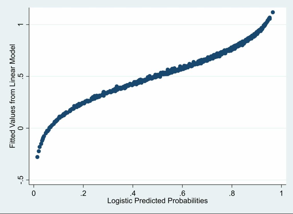
Notice that as the logistic predictions get close to 1, the linear predictions get larger than the logistic predictions. And, symmetrically, as the logistic predictions get close to 0, the linear predictions get smaller than the logistic predictions. This should alert us to the possibility that, even if none of the linear predicted values is outside the (0, 1) interval, the values at the two extremes may be biased in predictable ways.

By contrast, the plot below for LDM vs. logistic is very well calibrated.

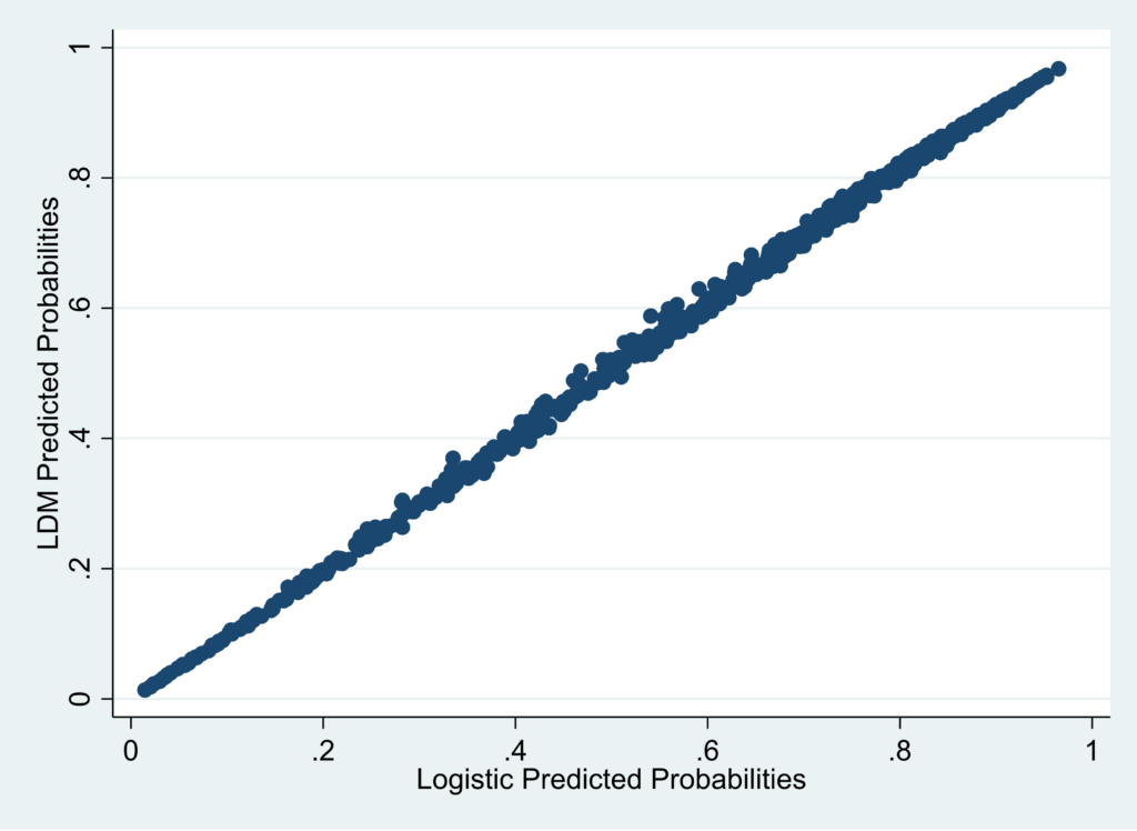
For this example, I’d say that very little would be lost in using the LDM predicted values instead of predicted values from conventional logistic regression. 

Example 2. All-Cause mortality among lung cancer patients

After deleting cases with missing data, there were 1,029 patients in the data set. Death is the dependent variable, and 764 of the patients died. What’s different about this example is that all the predictors are categorical and, therefore, have a joint distribution that is nothing like a multivariate normal. The predictors are surgery (1 or 0), a randomized treatment (1 or 0), hospital (Mayo Clinic, Johns Hopkins, or Sloan Kettering), and cancer stage at diagnosis (1, 2, or 3). Both of the 3-category variables are represented by two dummy (indicator) variables. The fitted models included main effects of these variables but no interactions.

Again, I ran two regressions, one linear and one logistic. The linear predictions were transformed by the LDM method. As the next table shows, there were definitely cases with linear predicted values greater than 1. In fact, there were 96 such cases.

    Variable |        Obs        Mean    Std. Dev.       Min        Max
-------------+---------------------------------------------------------
        yhat |      1,029    .7424684    .2206033   .4116536    1.01567
    yhat_ldm |      1,029    .7299414     .251858    .303894   .9679288
  yhat_logit |      1,029    .7424684    .2247691   .3621077   .9674457

Here are the correlations among the three versions of the predicted values.

             |     yhat yhat_ldm yhat_logit
-------------+---------------------------
        yhat |   1.0000
    yhat_ldm |   0.9754   1.0000
  yhat_logit |   0.9815   0.9908   1.0000

Again, the LDM predictions do a better job than the linear predictions of matching the conventional logistic predictions.

Conclusion

The LDM method is a simple and effective way to transform predicted values from a linear probability model so that they do not fall outside the (0,1) interval. Although the method relies on strong assumptions about the distribution of the predictor variables, it nevertheless performed very well in 13 out of 15 data sets and models that I have examined, none of which had predictors that came close to multivariate normality.

What about the two exceptions? Well, I’m still studying them to get a better understanding of what went wrong, but I can tell you this: In one of them, the model included a 2-way interaction that was highly significant in the linear model but not significant in the conventional logistic model. In the other, there were two predictors that were highly collinear. I am also designing a simulation study to explore the conditions under which the LDM method does or does not work well.

Is this a perfect method? Certainly not. I still prefer to use conventional logistic regression wherever computationally practical. But even with today’s enormous computing power, there are still many applications where linear models are quite attractive. And if you’re going to use an LPM and you want valid predicted probabilities, the LDM method seems like a pretty good way to get them.

References

Chatla, S. B., & Shmueli, G. (2017). An extensive examination of regression models with a binary outcome variable. Journal of the Association for Information Systems, 18(4), 1.

Fisher, R. A. (1936). The use of multiple measurements in taxonomic problems. Annals of eugenics, 7(2), 179-188.

Greene, W.H. (2017) Econometric Analysis. Pearson.

Haggstrom, G. W. (1983). Logistic regression and discriminant analysis by ordinary least squares. Journal of Business & Economic Statistics, 1(3), 229-238.

Hellevik, Ottar (2009): Linear versus logistic regression when the dependent variable is a dichotomy. Quality & Quantity 43.1 59-74.

Long, J. S. (1997) Regression models for categorical and limited dependent variables. Sage Thousand Oaks.

Mroz, T.A. (1987) “The sensitivity of an empirical model of married women’s hours of work to economic and statistical assumptions.” Econometrica 55: 765-799.

Press, S. J., & Wilson, S. (1978). Choosing between logistic regression and discriminant analysis. Journal of the American Statistical Association, 73(364), 699-705.

Westin, R. B. (1974). Predictions from binary choice models. Journal of Econometrics, 2(1), 1-16.

Wilensky, G. R., & Rossiter, L. F. (1978). OLS and logit estimation in a physician location study. In Proceedings of the Social Statistics Section, American Statistical Association (pp. 260-265).

Wooldridge, J. M. (2010). Econometric analysis of cross section and panel data. MIT press.

Appendix 1: Stata code for the examples

 Note: This program uses the predict_ldm command, which may be downloaded here.

 /*Example 1. 753 married women. DV=1 if in the labor force, else 0.*/

use "https://statisticalhorizons.com//www/wp-content/uploads/MROZ.dta",clear
reg inlf kidslt6 age educ exper expersq
predict_ldm
logit inlf kidslt6 age educ exper expersq
predict yhat_logit
sum yhat yhat_ldm yhat_logit
corr yhat yhat_ldm yhat_logit
scatter yhat yhat_logit, xtitle(Logistic Predicted Probabilities) ///
  ytitle(Fitted Values from Linear Model)
scatter yhat_ldm yhat_logit, xtitle(Logistic Predicted Probabilities) ///
  ytitle(LDM Predicted Probabilities)


/*Example 2. 1029 lung cancer patients. DV is 1 if patient died, else 0. */

use "https://statisticalhorizons.com//www/wp-content/uploads/lung.dta",clear
gen dead=surv!=0
reg dead operated treat i.instit i.stage
predict_ldm
logit dead operated treat i.instit i.stage
predict yhat_logit
sum yhat yhat_ldm yhat_logit
corr yhat yhat_ldm yhat_logit
scatter yhat yhat_logit
scatter yhat_ldm yhat_logit

Appendix 2:  SAS code for the examples

Note: This program uses the predict_ldm macro, which can be downloaded here. The data sets may be dowloaded here and here. 

/*Example 1. 753 married women. DV=1 if in the labor force, else 0.*/

%predict_ldm (data=my.mroz, y=inlf, x=kidslt6 age educ exper expersq);
proc logistic data=predict_ldm desc;
  model inlf=kidslt6 age educ exper expersq;
  output out=c pred=yhat_logit;
run;
proc corr data=c;
  var yhat yhat_ldm yhat_logit;
run;
proc gplot;
  plot yhat*yhat_logit;
  plot yhat_ldm*yhat_logit;
run;


/*Example 2. 1029 lung cancer patients. DV is 1 if patient died, else 0. */

data lung;
 set my.lung;
 dead=surv ne 0;
 hopkins=(instit=2);
 mayo=(instit=1);
 if stage=. then delete;
 stage3 = (stage=3);
 stage2 = (stage=2);
run;
%predict_ldm(data=lung, y=dead,
    x=operated treat hopkins mayo stage3 stage2);
proc logistic data=predict_ldm desc;
  model dead=operated treat hopkins mayo stage3 stage2;
  output out=c pred=yhat_logit;
run;
proc corr data=c;
  var yhat yhat_ldm yhat_logit;
run;
proc gplot data=c;
  plot yhat*yhat_logit;
  plot yhat_ldm*yhat_logit;
run;

 

Appendix 3:  R code for the examples 

# Function to convert linear predictions to the probability scale:
predict_ldm <- function(fit) {
  c <- fit$coefficients[1]
  k <- nrow( fit$model ) / deviance( fit )
  m <- mean( fit$model[,1] )
  a <- log(m/(1-m) ) + k*( c-.5 ) + .5*(1/m - 1/(1-m) )
  lin_preds <- predict(fit)
  my_preds_logit <- k*(lin_preds-c) + a
  my_preds <- 1/(1 + exp(-my_preds_logit))
  names(my_preds) <- "ldm_preds"
  return(my_preds)
}

# Example 1
library(haven)
library(psych)
mroz<-read_dta("https://statisticalhorizons.com//www/wp-content/uploads/MROZ.dta")
mroz_fit <- lm(inlf ~ kidslt6 + age + educ + exper + expersq, data = mroz)
summary(mroz_fit)
lin_preds <- predict(mroz_fit)
ldm_preds <-predict_ldm(mroz_fit)
logit_fit <- glm(inlf ~ kidslt6 + age + educ + exper + expersq,
                 family = binomial, data = mroz)
summary(logit_fit)
logit_preds <- predict(logit_fit, type = "response")
three_preds <- cbind(lin_preds, ldm_preds, logit_preds)
describe(three_preds, fast=T)
cor(three_preds)
plot(logit_preds,lin_preds)
plot(logit_preds, ldm_preds)
# Example 2
lung<-read_dta("https://statisticalhorizons.com//www/wp-content/uploads/lung.dta")
lung$dead<-(lung$surv!=0)
lung$i.stage <- as.factor(lung$stage)
lung$i.instit <- as.factor(lung$instit)
lung_fit <- lm(dead ~ treat+operated+i.stage+i.instit, data = lung)
summary(lung_fit)
lin_preds <- predict(lung_fit)
ldm_preds <-predict_ldm(lung_fit)
logit_fit <- glm(dead ~ treat+operated+i.stage+i.instit,
                 family=binomial, data = lung)
summary(logit_fit)
logit_preds <- predict(logit_fit, type = "response")
three_preds <- cbind(lin_preds, ldm_preds, logit_preds)
describe(three_preds, fast=T)
cor(three_preds)
plot(logit_preds,lin_preds)
plot(logit_preds, ldm_preds)