
For many years, one of the more popular ways of handling missing data was a technique known as dummy variable adjustment (DVA), a method designed to handle missing data on predictor variables in regression analysis (Cohen and Cohen 1975). It works with any kind of regression—linear, logistic, Cox, etc. And, as I will explain, it’s intuitive and easy to implement.
Unfortunately, it’s wrong. In a now-famous article, Michael Jones (1996), demonstrated that DVA (also known as the missing indicator method) generally yields biased estimates, even when data are missing completely at random. For this reason, contemporary reviews of missing data methods usually sweep DVA into the dustbin.
In this post, I’m going to pull it out. Although Jones performed an enormous service in showing us the pitfalls of DVA, I’ll argue that there are two situations in which DVA can be an effective missing data method, possibly better than my usual go-to methods of multiple imputation and (full information) maximum likelihood.
LEARN MORE IN A SEMINAR WITH PAUL ALLISON
Before we dive into that argument, let’s take a brief look at how DVA works. Suppose you want to do a linear regression of Y on two variables, X and Z, but there are a substantial number of cases that have missing values on X. You create a dummy (indicator) variable D that has a value of 1 if X is observed and 0 if X is missing. In addition, for the missing values of X, you substitute some constant value c. All three variables, X, Z, and D, then go into the regression as predictors.
In a fundamental sense, the model is invariant to the choice of c. In particular, the coefficients of X and Z will be the same no matter what c is. But the coefficient of D does depend on c. To facilitate interpretation of that coefficient, it’s often attractive to make c the mean of X for the non-missing cases.
Then, you just run the regression of Y on X, Z, and D. Done! That gives you estimates for the coefficients in this equation:
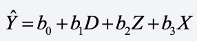
How are these coefficients interpreted?
- b2 is the effect of Z, controlling for everything we know about X.
- b3 is the effect of X on Y controlling for Z, among those with X observed.
- If c is the mean of X, b1 is the predicted value of Y for someone who is at the mean value of X minus the predicted value of Y for those who are missing on X.
In other words, the coefficient of the dummy for missingness tells us how much the missing cases differ on the dependent variable Y from an average individual who is not missing.
What if Z also has missing values? Then you just do the same things you did for X. You create another dummy variable that indicates whether or not Z is missing, and you plug in the mean of Z (or any other constant) for the missing values. The new dummy variable also goes into the regression. This can be extended to any number of predictors with missing data.
Here’s what’s attractive about this method:
- It’s not hard to do.
- It works with any kind of regression.
- No cases are lost.
- All the available information is incorporated into the regression model.
- The estimated standard errors will be accurate (if the usual assumptions about the error term are satisfied).
This last point is particularly noteworthy because many traditional methods (like pairwise deletion or single imputation) do a poor job of getting the standard errors right.
Unfortunately, as Jones showed, the coefficient estimates tend to be biased. Without going into the details of his proof, the intuition for this bias is pretty clear. If you substitute any constant value for the missing values of X, you’re reducing the true variability in that variable. If X and Z are correlated, that will lead to bias in the coefficient of Z. And that further induces bias in the coefficient of X.
This can happen even if the data are missing completely at random, and that makes DVA a non-starter. But wait! I’m now going to suggest two important situations in which Jones’s results do not rule out DVA.
1. Data are missing on X because that variable doesn’t apply or has no meaning for some subset of the sample.
An implicit assumption of Jones’s proof is that there are true values of X that are not observed and that have some impact on the dependent variable. But what if there are no such values?
Consider this typical example. Suppose you want to estimate a regression model in which Y is a measure of depression and X is a measure of marital satisfaction. However, 30% of the individuals in your sample are unmarried and, hence, their marital satisfaction is missing. Would it make any sense to do multiple imputation to impute their marital satisfaction? I think not.
Here’s an approach that makes more sense. Let’s assume that the data generating mechanism consists of two equations, one for married people and another for unmarried people:
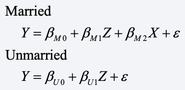
The obvious difference between these two equations is that X (marital satisfaction) does not appear in the equation for the unmarried people. The Z variable could be any other potential predictor of depression, say, education.
You could, of course, estimate these two equations separately for married and unmarried people. However, if you think that the effect of Z (or any other covariates) is the same for married and unmarried people, you’ll get much larger standard errors for the two separate estimates than if you had estimated a single estimate for both groups. Plus, if you have more than one “doesn’t apply” variable, you might have to estimate several different equations.
To fix this, let’s assume that the coefficient of Z is the same for both married and unmarried people, i.e.,
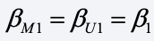
As before, we’ll let D = 1 if data are present for X (the married people), otherwise 0. Relying on a standard algebraic trick for combining equations for two groups using dummy variables, we get

This equation contains the “main effect” of D and the interaction of D and X. Multiplying X by D is equivalent to setting X to 0 when X is missing. But this is just the DVA model with c = 0. And if the ε satisfies the usual assumptions for linear regression, OLS applied to this model will yield “best unbiased estimates” of all coefficients.
Note also that for c = 0, the coefficient of D is the difference in the intercept for the original two equations for married and unmarried. On the other hand, if c is set equal to the sample mean of X, the coefficient of D has the interpretation described earlier. For this example, it would be the expected value of Y for married people who are at the mean of marital satisfaction minus the expected value of Y for those who are unmarried (controlling for any other variables in the model).
You could also add an interaction between Z and D, but that would be the equivalent of estimating the two equations separately (except that the error variances would be constrained equal).
The upshot is that DVA does a very good job of estimating the coefficients of a plausible model for the “doesn’t apply” situation. It’s hard to see how maximum likelihood or multiple imputation could improve on it. In fact, I did a small simulation which showed that DVA does a better job in this situation than either maximum likelihood or multiple imputation, both of which produced estimates that were substantially biased. (See Appendix 1 for details).
2. Missing data on baseline covariates in randomized controlled trials.
When analyzing data from a randomized controlled trial (RCT), it’s very common to estimate the treatment effect while controlling for one or more covariates that are measured at baseline, usually in an ANCOVA framework. Although a simple ANOVA would yield an unbiased estimate of the treatment effect, it’s desirable to include covariates in order to reduce the error variance in the model, thereby reducing the standard error of the treatment estimate. That, in turn, increases statistical power to test the treatment effect.
Baseline covariates often have missing data, however. It would be counterproductive to delete cases with missing data because that would tend to increase the standard errors, as well as violate the intention-to-treat principle. By contrast, DVA can be an effective method (Puma et al. 2009, Groenwold et al. 2012). As Jones noted in his original 1996 paper, bias only becomes a problem for DVA when the variable with missing data is correlated with other variables in the model. But in an RCT, baseline covariates are uncorrelated with the treatment by design. Consequently, DVA should not introduce any bias in the treatment effect.
But multiple imputation or maximum likelihood would also seem to be reasonable choices in the RCT situation. How does DVA compare with those methods? Again, I did a small simulation to compare the three methods for estimating the linear regression of Y on X and Z, when X and Z are uncorrelated. (See Appendix 2 for details).
In the simulation, Z is a dichotomous treatment indicator and X is a baseline covariate with missing data. The results showed that when data on X are missing completely at random, all three methods are approximately unbiased for the coefficients of both X and Z.
What about standard errors? As estimated by DVA, the standard error for the X coefficient was about 17% larger than those for maximum likelihood and multiple imputation. But we really don’t care about that coefficient. What we care about is the treatment effect, namely the coefficient of Z. For that coefficient, DVA yielded a smaller standard error than those for maximum likelihood or multiple imputation, although the differences were not large. The differences became substantially larger when X was not missing at random.
The upshot is that DVA seems to be at least as good, and possibly somewhat better, than maximum likelihood or multiple imputation for estimating the treatment effect for an RCT with baseline covariates that have missing data.
References
Cohen, J., and Cohen, P. (1975), Applied Multiple Regression Correlation Analysis for the Behavioral Sciences, New York John Wiley.
Groenwold, R. H., White, I. R., Donders, A. R. T., Carpenter, J. R., Altman, D. G., & Moons, K. G. (2012). “Missing covariate data in clinical research: when and when not to use the missing-indicator method for analysis.” Cmaj, 184(11), 1265-1269. https://doi.org/10.1503/cmaj.110977
Puma, Michael J., Robert B. Olsen, Stephen H. Bell, and Cristofer Price (2009). “What to Do When Data Are Missing in Group Randomized Controlled Trials” (NCEE 2009-0049). Washington, DC: National Center for Education Evaluation and Regional Assistance, Institute of Education Sciences, U.S. Department of Education. https://ies.ed.gov/pubsearch/pubsinfo.asp?pubid=NCEE20090049
Appendix 1. Simulation to Evaluate DVA for “does not apply” applications.
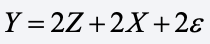
Data were generated based on the model shown above for married and unmarried people. Specifically,

where X and Z are both standard normal with a correlation of 0.50. In both equations, ε is standard normal and independent of X and Z.
Because I was only concerned about bias, not sampling variation, I generated a single large sample, with 10,000 married and 10,000 unmarried. X was then made to be missing (completely at random) with a probability of 0.50.
The next step was to estimate the regression of Y on X and Z, using three different methods: DVA, multiple imputation, and full information maximum likelihood. All data generation and analysis were done with R.
For DVA, I just used the lm function. I used the lavaan package for maximum likelihood and the jomo package for multiple imputation (25 data sets imputed via the multivariate normal MCMC method). R code is shown below.
Here are the results.
| DVA | Maximum Likelihood | Multiple Imputation |
| Variable | Estimate | S.E. | Estimate | S.E. | Estimate | S.E. |
| X | 2.010 | .020 | 1.846 | .019 | 1.844 | .019 |
| Z | 2.006 | .015 | 1.780 | .017 | 1.781 | .017 |
Since the true coefficients were both 2.0, it’s clear that DVA is producing approximately unbiased results. As expected, maximum likelihood and multiple imputation produced estimates that were very similar to each other. However, both sets of estimates were about 8 to 10% lower than the true values.
This simulation should only be regarded as exploratory. I only used one set of parameter values, a single covariate, a strictly linear model, and a single missing data mechanism. Nevertheless, it strongly suggests that multiple imputation and maximum likelihood may yield biased estimates for a plausible “does not apply” model.
R Code for “Does Not Apply” Simulation
#Appendix 1
library(lavaan)
library(jomo)
library(mitools)
library(mice)

#Generate data
set.seed(3495)
n <- 10000
z_mar <- rnorm(n)
x_mar <- .5*z_mar + sqrt(1-.5*.5)*rnorm(n)
y_mar <- 3 + 2*z_mar + 2*x_mar + 2*rnorm(n)
z_sing <- rnorm(n)
x_sing <- rep(NA, n)
y_sing <-  4 + 2*z_sing + 2*rnorm(n)
dat <- data.frame(y=c(y_mar, y_sing),
                 z=c(z_mar, z_sing),
                 x=c(x_mar, x_sing))
dat$d <- ifelse(is.na(dat$x), 0, 1)
dat$x.dva <- ifelse(is.na(dat$x), 0, dat$x)

#DVA method
mod.dva <- lm(y ~ x.dva + z + d, data=dat)
summary(mod.dva)

#Maximum likelihood
mod.ml <- sem('y ~ x + z', data=dat, missing='fiml.x')
summary(mod.ml)

#Multiple imputation
datsub <- subset(dat,select=-c(d,x.dva))
outjomo <-jomo(datsub, nimp=25)
mi_list <- imputationList(split(outjomo, outjomo$Imputation)[-1])
mi_results <- with(mi_list, lm(y ~ x + z))
summary(pool(as.mira(mi_results)),type="all")
Appendix 2. Simulation to Evaluate DVA for RCTs.
I generated data according to the model
where Z is a treatment indicator with values of 1 and 0, each with probability 0.50. Both X and ε are standard normal variates, independent of each other and of Z. I then made X missing (completely at random) with probability 0.50.
In order to get model-free estimates of the standard errors, I generated 1,000 samples, each of size 200. For each sample, the model was estimated by DVA, maximum likelihood and multiple imputation.
All data generation and analysis were done with R. For DVA, I just used the built-in lm function. I used the lavaan package for maximum likelihood and the jomo package for multiple imputation (10 data sets per sample). Both maximum likelihood and multiple imputation were based on the multivariate normal assumption, which is satisfied for these data by design. R code is shown below.
The following table reports the means of the coefficient estimates and the standard deviations (estimated standard errors) of those estimates across the repeated samples.
| DVA | Maximum Likelihood | Multiple Imputation |
| Variable | Estimate | S.E. | Estimate | S.E. | Estimate | S.E. |
| X | 1.987 | .209 | 2.011 | .177 | 1.975 | .180 |
| Z | 2.004 | .340 | 1.998 | .344 | 1.979 | .345 |
All three methods appear to be approximately unbiased for the coefficients of both X and Z. Maximum likelihood and multiple imputation produced noticeably smaller standard errors than DVA for the coefficient of X. But, as already noted, we don’t care about that coefficient. For the treatment effect, DVA has the smallest standard error, although the differences are not large and may well be within the range of Monte Carlo error.
I then switched things up to make X not missing at random, and in an extreme way. Specifically, all values of X less than 0 were missing, and all values greater than 0 were observed. That changed the results in an unexpected way:
| DVA | Maximum Likelihood | Multiple Imputation |
| Variable | Estimate | S.E. | Estimate | S.E. | Estimate | S.E. |
| X | 1.997 | .346 | 2.612 | .333 | 2.519 | .339 |
| Z | 1.987 | .296 | 1.995 | .377 | 1.981 | .376 |
Now, the coefficients for X are unbiased for DVA but clearly biased upward for maximum likelihood and multiple imputation (by about 30%). All three methods are approximately unbiased for the treatment effect, but DVA has a standard error more than 20% lower than the other two.
This simulation should only be regarded as exploratory. I only used one set of parameter values, a single sample size, a single covariate, a strictly linear model, and only two missing data mechanisms. But, at the least, it should tell us that DVA is a strong contender for dealing with missing baseline covariate values in RCTs.
R Code for RCT Simulation
#Appendix 2
library(lavaan)
library(jomo)
library(mitools)
library(mice)
library(psych)
set.seed(23599)

#MCAR Scenario

#Create empty data frames to hold coefficients
dva <- data.frame(matrix(ncol = 4, nrow = 0))
   colnames(dva) <-c("(Intercept)", "x.dva","z","d")
ml <- data.frame(matrix(ncol = 4, nrow = 0))
   colnames(ml) <-c("y~x", "y~z","y~~y","y~1")
mult <- data.frame(matrix(ncol = 3, nrow = 0))
   colnames(mult) <-c("(Intercept)", "x","z")

for (i in 1:1000) {
  #Generate MCAR Data
  n <- 200
  z <- as.numeric(rnorm(n)>0)
  x <- rnorm(n)
  y <- 2*z + 2*x + 2*rnorm(n)
  xmiss <- ifelse(rnorm(n)<0,NA,x)
  dat <- data.frame(y=y,x=xmiss,z=z)

  #DVA method
  dat$d <- ifelse(is.na(dat$x), 0, 1)
  dat$x.dva <- ifelse(is.na(dat$x), 0, dat$x)
  mod.dva <- lm(y ~ x.dva + z + d, data=dat)
  dva[nrow(dva) + 1,] <- mod.dva$coefficients

  #Maximum likelihood
  mod.ml <- sem('y ~ x + z', data=dat, missing='fiml.x')
  ml[nrow(ml) + 1,] <- coef(mod.ml)

  #Multiple imputation
  datsub <- subset(dat,select=-c(d,x.dva))
  outjomo <-jomo(datsub, nimp=10, nburn=100, nbetween=20, output=2)
  mi_list <- imputationList(split(outjomo, outjomo$Imputation)[-1])
  mi_results <- with(mi_list, lm(y ~ x + z))
  mult[nrow(mult) + 1,] <- getqbar(pool(as.mira(mi_results)))
}

print(describe(dva, fast=T),digits=3)
print(describe(ml, fast=T),digits=3)
print(describe(mult, fast=T),digits=3)


#NMAR scenario

set.seed(4321)
#Create empty data frames to hold coefficients
dva <- data.frame(matrix(ncol = 4, nrow = 0))
  colnames(dva) <-c("(Intercept)", "x.dva","z","d")
ml <- data.frame(matrix(ncol = 4, nrow = 0))
  colnames(ml) <-c("y~x", "y~z","y~~y","y~1")
mult <- data.frame(matrix(ncol = 3, nrow = 0))
  colnames(mult) <-c("(Intercept)", "x","z")

for (i in 1:1000) {
  #Generate NMAR Data
  n <- 200
  z <- as.numeric(rnorm(n)>0)
  x <- rnorm(n)
  y <- 2*z + 2*x + 2*rnorm(n)
  xmiss <- ifelse(x<0,NA,x)
  dat <- data.frame(y=y,x=xmiss,z=z)

  #DVA method
  dat$d <- ifelse(is.na(dat$x), 0, 1)
  dat$x.dva <- ifelse(is.na(dat$x), 0, dat$x)
  mod.dva <- lm(y ~ x.dva + z + d, data=dat)
  dva[nrow(dva) + 1,] <- mod.dva$coefficients

  #Maximum likelihood
  mod.ml <- sem('y ~ x + z', data=dat, missing='fiml.x')
  ml[nrow(ml) + 1,] <- coef(mod.ml)

  #Multiple imputation
  datsub <- subset(dat,select=-c(d,x.dva))
  outjomo <- jomo(datsub, nimp=10, nburn=100, nbetween=20, output=2)
  mi_list <- imputationList(split(outjomo, outjomo$Imputation)[-1])
  mi_results <- with(mi_list, lm(y ~ x + z))
  mult[nrow(mult) + 1,] <- getqbar(pool(as.mira(mi_results)))
}

print(describe(dva, fast=T),digits=3)
print(describe(ml, fast=T),digits=3)
print(describe(mult, fast=T),digits=3)