
Measurement invariance is a big deal in psychometrics—and in many related fields. In this post, I’m going to argue that the traditional approach to testing for measurement invariance is often more complicated than necessary. Instead, I’ll show how MIMIC models provide a shortcut that is both easier and often more instructive.
So, what is measurement invariance and why should we care about it? Suppose, for example, that you want to compare mean levels of depression for men and for women. Unless your measure of depression is fundamentally “the same” across the two groups, any conclusions that you draw may well be invalid. But how do you determine whether your measuring instrument is the same for the two groups? How do you even define invariance?
LEARN MORE IN A SEMINAR WITH MATTHEW DIEMER
For variables like depression that are typically measured by multiple-item scales, the traditional approach to invariance has been to estimate a confirmatory factor model in each group. Invariance is then defined by the extent to which different components of those models are the same across groups. There are four levels of invariance:
- Configural – The basic structure of the model is the same in each group. In other words, if you draw a path diagram of the model, it will look (i.e., be “configured”) the same for each group.
- Metric – Configural invariance, plus the factor loadings are the same in each group.
- Scalar – Metric invariance, plus the item intercepts are the same in each group.
- Strict invariance – Scalar invariance, plus the error variances of the items are the same in each group.
Strict invariance is the ideal, but it’s rarely achieved. Fortunately, there are many situations where the goals of your study can be satisfied by having only scalar invariance, or even just metric invariance. Unfortunately, the whole process of testing whether these different levels of invariance have been achieved can be complex and tedious.
Enter MIMIC models. The acronym stands for multiple indicators, multiple causes. MIMIC models are well known in the structural equation modeling literature. They’ve been around for a long time, and they’ve been used for many different purposes. Here we’ll see how MIMICs can detect bias across groups in how observed indicators measure latent constructs.
A MIMIC model typically has three parts:
- A latent variable.
- Two or more observed indicators of the latent variable (at least three are needed for testing measurement invariance).
- One or more “exogenous” variables that affect the latent variable.
See Figure 2 below for a path diagram of the MIMIC model that we’ll use in the example.
MIMIC models combine features of confirmatory factor analysis (CFA) and structural equation modeling (SEM) in order to test whether groups of interest have similar latent means and similar responses to observed items (after adjusting for group differences in the latent means) (Gallo, Anthony & Muthén, 1994; Kaplan, 2008). Formally, MIMICs test for scalar invariance, or whether item intercepts are equivalent after adjusting for any latent mean differences (Putnick & Bornstein, 2016).
Scalar invariance indicates that groups that have the same (after adjustment) latent mean will have similar responses to the items that measure that latent construct. For example, after you adjust for differences between latent depression for men and women, scalar invariance indicates that men and women should give similar responses to individual items assessing mood. Scalar invariance is considered a “strong” form of measurement invariance that establishes whether the scaling of responses is measured in the same way and means the same thing across groups (Putnick & Bornstein, 2016).
On the other hand, if responses to items systematically vary across groups, after adjusting for latent mean differences between groups, then we have evidence of differential item functioning, or DIF (Kaplan, 2008). DIF is generally associated with item response theory, yet DIF can more easily be parameterized and tested in a MIMIC model.
The relatively simple MIMIC specification yields complex claims about group bias in measurement, which makes their underutilization surprising. In addition to their simplicity, MIMIC models have lower sample size requirements–you don’t need to divide a sample into multiple groups (as you do in measurement invariance testing) in order to test for measurement equivalence across groups of interest. This is particularly important in studies of minoritized, hard-to-recruit, low-incidence, and/or geographically mobile populations.
Three Steps in Specifying and Testing MIMIC Models
MIMIC models can be estimated in many SEM packages (e.g., R/lavaan, Stata, MPlus, SAS), with results obtained from different packages highly convergent (Chang et al., 2020; Diemer et al., 2023). The relatively simple specification and testing of MIMIC models can be partitioned into three sequential steps.
The first step is to develop a well-fitting CFA model for the sample as a whole, such that model fit indices meet commonly agreed upon cutoffs and items load significantly and with sufficient magnitude. Going the extra mile to examine measurement quality in this way provides important evidence of construct validity, beyond what Cronbach’s alpha and other estimates of internal consistency tell you. An example is depicted in Figure 1. (Note: Error terms are not included in the diagrams).
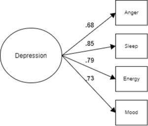
Figure 1. A CFA Model for Depression (Step 1).
The second step incorporates aspects of structural equation modeling by including a binary exogeneous covariate as a predictor of the latent variable. This covariate represents the groups to be compared by way of dummy coding (e.g., men = 0 and women = 1). If the covariate significantly predicts the latent variable, that indicates a difference in the latent variable means for the two groups. An example is depicted in Figure 2.
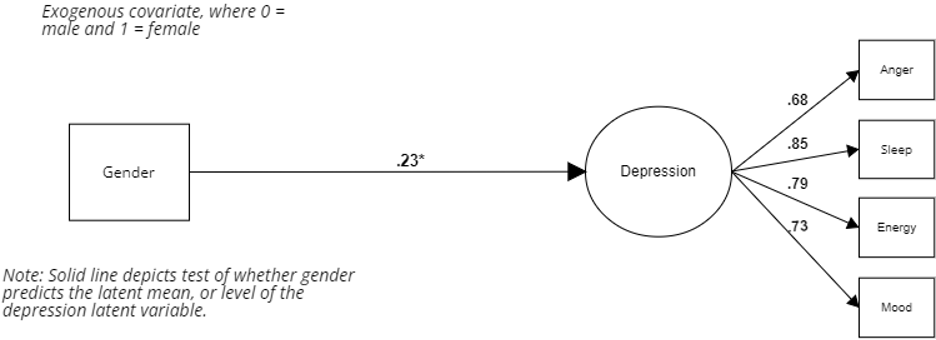
Figure 2. A MIMIC Model for Depression (Step 2).
The third step retains the regression of the latent variable on the exogenous covariate while also regressing individual items on the covariate. This step gives us the test of scalar invariance, i.e., whether item intercepts are invariant across the two groups. An example is depicted in Figure 3.

Figure 3. Modified MIMIC Model for Depression (Step 3).
A Practical Example: Gender Differences in Depression
Let’s return to Figure 1, which depicts a latent variable called depression which, in turn, predicts four observed indicators: anger, sleep, energy, and mood. (This is a manufactured example. For an example with real data and associated code, see Diemer et al. (2023) ). As per standard convention, the latent variable is enclosed by a circle while the observed variables are enclosed by rectangles. The values .68, .85, .79, and .73 are the standardized factor loadings of each item onto the depression latent variable. Testing how well depression is measured by these four indicators corresponds to step one in the MIMIC process.
In Figure 2, we add an exogeneous covariate (gender as a 0/1 binary variable) that predicts the latent depression variable. We have a significant difference in the latent mean of depression – reflected in the .23 standardized coefficient in the Figure. Because women are coded 1 for the covariate, this coefficient tells us that women have a significantly higher mean level of depression than men. This path corresponds to step two in the MIMIC process.
In step three, the path from the covariate to the latent variable is retained, in order to adjust the latent means to be equal when testing for differences in the observed items that measure the latent variable. This is depicted in Figure 3. In this case, the -.15 standardized coefficient from the exogeneous covariate to the anger observed indicator is an example of what we’d call a biased item – here the anger indicator systematically undermeasures anger for women.
Stated another way, even after adjusting the latent means of men and women to be equal, women with equivalent levels of depression to men are less likely to endorse anger. If the anger item was scaled 1-5, for example, then men with higher levels of depression might choose a 4 for the anger item – while women with a similar level of depression may choose a 3 for the anger item.
This systematic pattern of difference in how item scaling is interpreted represents DIF, in this case non-invariance in the intercepts for the anger item. By extension, this measure would underestimate the level of depression in women – which could then bias estimates derived from this measure. For example, if you wanted to use the depression measure to predict alcohol use, failure to account for DIF could incorrectly make it look like depression had different effects for men and for women.
Extensions and Caveats
Although we have only considered a comparison of two groups, the MIMIC approach can easily be extended to three or more groups. For three groups, you would need two exogenous covariates with dummy coding to represent those groups, and so on.
One disadvantage of the MIMIC approach is that it presumes that metric invariance (equal factor loadings for the groups) has already been achieved. The (quite advanced) non-uniform DIF approach can test factor loadings in a MIMIC model, but loses the simplicity of the MIMIC (Woods & Grimm, 2011). The capacity of MIMIC models to detect non-invariance in intercepts, when there is non-invariance in the slopes, is an open question. Thus, MIMIC models could provide evidence for DIF even if metric invariance doesn’t hold.
Another caveat is that you can’t test for DIF in all the items at once. It’s easy to include direct effects from the exogeneous covariate to too many observed indicators, in which case the model will not be identified. At most it can have direct effects on all but one item (and the choice of that item would be arbitrary). In practice, it’s probably better to test one item at a time, sequentially.
Summary
The ability to detect item bias is a powerful feature of MIMIC models, and one with important equity implications (see Diemer et al., 2023 for more on this). Further, in a full structural equation modeling specification, paths from the covariate to the latent mean and to items exhibiting DIF can be retained, to adjust for and “explain away” intercept bias in items when subsequently estimating regression relations among latent constructs (Gallo et al., 1994). Despite these advantages, and their relative simplicity, MIMICs are not used as often as they should be. Hopefully, this post illustrates what MIMICs can accomplish, how to specify them, and how to interpret then – encouraging more people to use them.
References
Chang, C., Gardiner, J., Houang, R., & Yu, Y. L. (2020). Comparing multiple statistical software for multiple-indicator, multiple-cause modeling: an application of gender disparity in adult cognitive functioning using MIDUS II dataset. BMC Medical Research Methodology, 20, 1-14. https://doi.org/10.1186/s12874-020-01150-4
Diemer, M.A., Frisby, M.B., Marchand, A.D & Bardelli, E. (2023). Illustrating and enacting a Critical Quantitative approach to measurement with MIMIC models. Manuscript under review. https://psyarxiv.com/8thpu
Gallo, J. J., Anthony, J. C., & Muthén, B. O. (1994). Age differences in the symptoms of depression: A latent trait analysis. Journal of Gerontology, 49(6), 251-264. https://doi.org/10.1093/geronj/49.6.P251
Kaplan, D. (2008). Structural equation modeling: Foundations & extensions. Thousand Oaks, CA: Sage Publications.
Putnick, D. L., & Bornstein, M. H. (2016). Measurement invariance conventions and reporting: The state of the art and future directions for psychological research. Developmental Review, 41, 71-90. https://doi.org/10.1016/j.dr.2016.06.004
Woods, C.M. & Grimm, K.J. (2010). Testing for nonuniform differential item functioning with Multiple Indicator Multiple Cause Models. Applied Psychological Measurement, 35(5), 339-361. https://doi.org/10.1177/0146621611405984
*Thanks to Emanuele Bardelli, Michael Frisby and Aixa Marchand, for ideas and insights that shaped this blog post.