
In July 2015 I pointed out some advantages of the linear probability model over the logistic model. The linear model is much easier to interpret, and the linear model runs much faster, which can be important if the data set is large or the model is complicated. In addition, the linear probability model often fits about as well as the logistic model, since over some ranges the probability p is almost linearly related to the log odds function ln(p(1-p)) that is used in logistic regression.
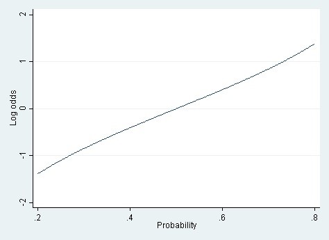
As a rule of thumb I suggested that the linear probability model could be used whenever the range of modeled probabilities is between .20 and .80. Within that range the relationship between the probability and the log odds is almost linear.
LEARN MORE IN ONE OF OUR SHORT SEMINARS
Figure 1. The relationship between probability and log odds over the range of probabilities from .2 to .8.
This is reasonable advice, and similar advice has been given before (Long, 1997). But it doesn’t go far enough. There is a wider range of circumstances where the linear probability model is viable.
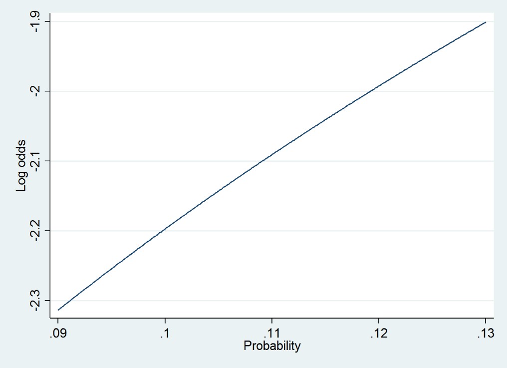
For example, in a new paper Joe Workman and I used a multilevel model to analyze obesity among US children in kindergarten through 2nd grade—an age range over which the probability of obesity increases from .09 to .13. Since these probabilities are less than .20, you might guess that we couldn’t use the linear probability model. But we could, and we did. The linear model ran very quickly, whereas the logistic model can be slow when used in a multilevel context. The linear model also gave us very interpretable results; for example, we could write that “during the summer, children’s probability of obesity increases by approximately 1 percentage point per month.” And we didn’t lose any sleep about model fit; the linear model fit practically as well as a logistic model, because over the range of probabilities from .09 to .13 the probability is almost linearly related to the log odds.
Figure 2. The relationship between probability and log odds over the range of probabilities from .09 to .13.
The basic insight is that the linear probability model can be used whenever the relationship between probability and log odds is approximately linear over the range of modeled probabilities. Probabilities between .2 and .8 are one range where approximate linearity holds—but it also holds for some narrow ranges of probabilities that are less than .2 or greater than .8.
I still haven’t gone far enough. When the relationship between probability and log odds is nonlinear, there are still situations where the linear probability model is viable. For example, if your regressors X are categorical variables, then you’re not really modeling a continuous probability function. Instead, you’re modeling the discrete probabilities associated with different categories of X, and this can be done about as well with a linear model as with a logistic model—particularly if your model includes interactions among the X variables (Angrist & Pischke, 2008, chapter 3; Pischke, 2012).
I don’t think that the linear probability model is always viable. I do use the logistic model sometimes. For example, looking at 30 years of data from the Belmont Stakes horse race, I found that the probability of an upset was strongly related to the number of horses that started the race. The more horses started, the more likely it became that one of them would upset the favorite. The relationship looked like this.[1]
Figure 3. The relationship between the number of horses starting the Belmont Stakes and the probability that the favorite will be upset.
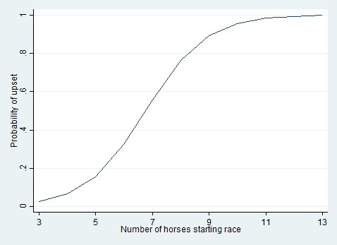
On a probability scale the relationship is strongly nonlinear. It almost has to be, because the relationship is strong and the probabilities cover almost the full range from 0 to 1. A linear probability model can’t fit these data easily. When I tried a linear model, out of curiosity, I found that some of the modeled probabilities were out of bounds—greater than 1. I could improve the fit of the linear model by subjecting the X variable to some nonlinear transformation, but finding the right transformation isn’t trivial, and even if I found it the linear model’s ease of interpretation would be lost. It’s simpler to fit a logistic model which naturally keeps the probabilities in bounds.
To check whether your data are candidates for a linear probability model, then, a basic diagnostic is to plot the relationship between probability and log odds over the likely range of probabilities in your data. If the relationship is nearly linear, as in Figures 1 and 2, then a linear probability model will fit about as well as a logistic model, and the linear model will be faster and easier to interpret. But if the relationship is strongly nonlinear, as in Figure 3, then a linear model may fit poorly—unless your Xs are categorical.
The relationship between probability and log odds is easy to plot in a variety of software. In Stata, for example, I plotted the relationship in Figure 1 with a single command, as follows:
twoway function y=ln(x/(1-x)), range(.2 .8) xtitle(“Probability”) ytitle(“Log odds”)
I plotted Figure 2 using the same command, only changing the range to (.09 .13).
In some situations, the relationship between probability and log odds is slightly but not severely nonlinear. Then you face a tradeoff, and your choice of model will depend on your goals. If what you mainly want is a rough but clear summary of the relationships, you might be willing to tolerate a bit of misfit and use a linear model that runs quickly and gives coefficients that are easy to interpret. But if you really want to get the probabilities just right, then you might be willing to sacrifice runtime and interpretability for better probability estimates. For example, I’ve developed financial risk models that predict the probability that a transaction is fraudulent or a borrower will default. In that situation, the coefficients are not the focus. What you really want the model to do is assign accurate probabilities to individual transactions or borrowers, and the linear model often does that poorly over the range of probabilities that are typical for a risk model. Then the logistic model is a more natural choice, although other nonlinear models, such as neural networks or classification trees, are also used.
Paul von Hippel is an Associate Professor in the LBJ School of Public Affairs at the University of Texas, Austin, with affiliations and courtesy appointments in Sociology, Population Research, and Statistics and Data Science.
References
Angrist, J. D., & Pischke, J.-S. (2008). Mostly Harmless Econometrics: An Empiricist’s Companion (1st ed.). Princeton University Press.
Long, J. S. (1997). Regression Models for Categorical and Limited Dependent Variables (1st ed.). Sage Publications, Inc.
Pischke, J.-S. (2012, July 9). Probit better than LPM? Retrieved from http://www.mostlyharmlesseconometrics.com/2012/07/probit-better-than-lpm/
von Hippel, P.T. & Workman, J. (2016). From Kindergarten Through Second Grade, U.S. Children’s Obesity Prevalence Grows Only During Summer Vacations. Obesity Volume 24, Issue 11, pages 2296–2300. http://onlinelibrary.wiley.com/doi/10.1002/oby.21613/full
[1] The relationship looked a little different in my original article on the Belmont Stakes. In that article I constrained the modeled probabilities to reflect the assumption that the probability of an upset cannot exceed n/(n-1) where n is the number of starters. I also subjected the regressor to a reciprocal transformation, but this made less of a difference to the modeled probabilities.
Comments
I agree that the linear probability model has advantages and is sometimes called for, based on theoretical and statistical grounds. Sometimes the theory of functional form of the relationship between P(y) and x calls for the linear probability model. When the functional form differs between P(y) and the x variables in multivariate models, the different forem can often be accomodated within the linear probability framework (e.g. using x and x-squared, etc). Logistic regression tends to be used within health and social sciences when analyzing dichotomous outcomes, usually without any justification. It should be noted that there is a linearity test that could be used within the linear probability framework (using WLS regression) to test whether the linearity assumption holds (see Kim & Kohout, 1975. p. 376-377). I myself used this test to assess linearity in the relationship between negative life events and clinical depression (Vilhjalmsson, 1993, p. 339). A significant test however does not tell what kind of nonlinearity is the correct functional form of the relationship between P(y) and x.
References:
Kim, J.-O., & Kohout, F. J. (1975). Special topics in general linear models. In N. N. Nie, C. H Hull, J. G. Jenkins, K. Steinbrenner, & D. H. Brent (eds.), Statistical Package for the Social Sciences, 2nd ed. NY: McGraw-Hill.
Vilhjalmsson, R (1993). Life stress, social support and clinical depression: A reanalysis of the literature. Social Science and Medicine, 37, 331-342.
Thanks for this, Paul. Just a few additional points worth making
1. Probably best to use robust estimator (e.g., Huber-White) when aplying the LPM to deal with heteroscedascity – as you note in your first post. I like to refer to this as the modified linear probability model (MLPM) to keep it distinct from the traditional LPM that relies on OLS. It generally outperforms OLS based LPM.
2. In the 40 years I have been analyzing data, I have rarely come across an S shaped logit function linking continuous predictors to probabilities of an outcome. The S function is idealized that everyone seems to assume is descriptive of the data. Your advice to explore the operating functions in the data first is solid, i.e., determine if a logit function is, in fact, viable; determine if a linear function is viable, etc. and then model accordingly
3. If we have 2 continuous predictors (X1 and X2) and one is linearly related to the outcome probabilities and the other is quadratically related, in the MLPM it is straightforward to deal with this; use X1 + X2 + x2^2 as predictors (or spline modeling for X2). Dealing with this case would be a nightmare in a logistic framework. The general point is that logistic regression assumes all continuous predictors are S shaped related to outcome probabilities across the full range of probability. In reality, the functions might differ for different predictors and depending on the range of probabilities in the data. To me, it is far easier to start with a linear function as a basis and then make adjustments to the predictors (transformations, polynomials, splines) to accommodate different types of non-linearity for each predictor instead of starting with an S function as a basis and trying to make it work. As Angrist states, the S function is just as arbitrary as a linear function but the latter is often much easier to work with.
4. Using MLPM instead of logit makes many types of modeling (mediation, instrumental variables, fixed effects) much more straight-forward then the gymnastics required by logit or probit models. Granted, these things can often be pulled off with logit, but you often end up in basically the same place as the MLPM