
In my last post, I explained several reasons why I prefer logistic regression over a linear probability model estimated by ordinary least squares, despite the fact that linear regression is often an excellent approximation and is more easily interpreted by many researchers.
I addressed the issue of interpretability by arguing that odds ratios are, in fact, reasonably interpretable. But even if you hate odds ratios, you can still get estimates from a logistic regression that have a probability interpretation. In this post, I show how easy it is to do just that using the margins command in Stata. (It’s even easier with the SPost13 package for Stata by Long & Freese).
If you want to do this sort of thing in R, there’s a package that just came out called margins. It’s modeled after the margins command in Stata but doesn’t have all its capabilities. For SAS users, there is an official SAS document on methods for calculating marginal effects. (This is reasonably easy for PROC QLIM but takes a discouraging amount of programming for PROC LOGISTIC.)
LEARN MORE IN A SEMINAR WITH PAUL ALLISON
I’ll continue using the NHANES data set that I used in the last post. As previously noted, that data set is publicly available on the Stata website and can be directly accessed from the Internet within a Stata session. (I am indebted to Richard Williams for this example. You can get much more detail from his PowerPoint presentation available here.)
There are 10,335 cases with complete data on the variables of interest. I first estimated a logistic regression model with diabetes (coded 1 or 0) as the dependent variable. Predictors are age (in years) and two dummy (indicator) variables, black and female. The Stata code for estimating the model is
   webuse nhanes2f, clear
   logistic diabetes i.black i.female age
The i. in front of black and female tells Stata to treat these as categorical (factor) variables. Ordinarily, this wouldn’t be necessary for binary predictors. But it’s important for getting Stata to calculate marginal effects in an optimal way.
Here are the results:
------------------------------------------------------------------------------
    diabetes | Odds Ratio   Std. Err.      z    P>|z|     [95% Conf. Interval]
-------------+----------------------------------------------------------------
     1.black |   2.050133   .2599694     5.66   0.000     1.598985     2.62857
    1.female |   1.167141   .1100592     1.64   0.101     .9701892    1.404074
         age |   1.061269    .003962    15.93   0.000     1.053532    1.069063
       _cons |   .0016525    .000392   -27.00   0.000     .0010381    .0026307
------------------------------------------------------------------------------
A typical interpretation would be to say that the odds of diabetes is twice as large for blacks as for non-blacks, an “effect” that is highly significant. Females have a 17% higher odds of diabetes than males, but that’s not statistically significant. Finally, each additional year of age is associated with a 6% increase in the odds of diabetes, a highly significant effect.
Now suppose we want to estimate each variable’s effect on the probability rather than odds of diabetes. Here’s how to get what’s called the Average Marginal Effect (AME) for each of the predictors:
margins, dydx(black female age)
yielding the output
------------------------------------------------------------------------------
             |            Delta-method
             |      dy/dx   Std. Err.      z    P>|z|     [95% Conf. Interval]
-------------+----------------------------------------------------------------
     1.black |   .0400922   .0087055     4.61   0.000     .0230297    .0571547
    1.female |   .0067987   .0041282     1.65   0.100    -.0012924    .0148898
         age |   .0026287   .0001869    14.06   0.000     .0022623    .0029951
------------------------------------------------------------------------------
The dy/dx column gives the estimated change in the probability of diabetes for a 1-unit increase in each predictor. So, for example, the predicted probability of diabetes for blacks is .04 higher than for non-blacks, on average.
How is this calculated? For each individual, the predicted probability is calculated in the usual way for logistic regression, but under two different conditions: black=1 and black=0. All other predictor variables are held at their observed values for that person. For each person, the difference between those two probabilities is calculated, and then averaged over all persons. For a quantitative variable like age, the calculation of the AME is a little more complicated.
There’s another, more traditional, way to get marginal effects: for the variable black, hold the other two predictors at their means. Then calculate the difference between the predicted probabilities when black=1 and when black=0. This is called the Marginal Effect at the Means (MEM). Note that calculation of the MEM requires only the model estimates, while the AME requires operating on the individual observations.
We can get the MEM in Stata with the command:
margins, dydx(black female age) atmeans
with the result
------------------------------------------------------------------------------
             |            Delta-method
             |      dy/dx   Std. Err.      z    P>|z|     [95% Conf. Interval]
-------------+----------------------------------------------------------------
     1.black |   .0290993   .0066198     4.40   0.000     .0161246    .0420739
    1.female |   .0047259   .0028785     1.64   0.101    -.0009158    .0103677
         age |   .0018234   .0000877    20.80   0.000     .0016516    .0019953
------------------------------------------------------------------------------
Here the MEM for black is noticeably smaller than the AME for black. This is a consequence of the inherent non-linearity of the model, specifically, the fact that averaging on the probability scale (the AME) does not generally produce the same results as averaging on the logit scale (the MEM).
The non-linearity of the logistic model suggests that we should ideally be looking at marginal effects under different conditions. Williams (and others) refers to this as Marginal Effects at Representative Values.
Here’s how to get the AME for black at four different ages:
margins, dydx(black) at(age=(20 35 50 65))
1._at        : age             =          20
2._at        : age             =          35
3._at        : age             =          50
4._at        : age             =          65
------------------------------------------------------------------------------
             |            Delta-method
             |      dy/dx   Std. Err.      z    P>|z|     [95% Conf. Interval]
-------------+----------------------------------------------------------------
1.black      |
         _at |
          1  |   .0060899   .0016303     3.74   0.000     .0028946    .0092852
          2  |   .0144831   .0035013     4.14   0.000     .0076207    .0213455
          3  |   .0332459   .0074944     4.44   0.000      .018557    .0479347
          4  |   .0704719    .015273     4.61   0.000     .0405374    .1004065
------------------------------------------------------------------------------
We see that the AME of black at age 20 is quite small (.006) but becomes rather large (.070) by age 65. This should not be thought of as an interaction, however, because the model says that the effect on the log-odds (logit) is the same at all ages.
Would it make sense to apply the linear probability model to these data? Von Hippel advises us to plot the log-odds versus the range of predicted probabilities and check whether the graph looks approximately linear. To get the predicted probabilities and their range, I used
   predict yhat
   sum yhat
The predict command generates predicted probabilities and stores them in the variable yhat. The sum command produces descriptive statistics for yhat, including the minimum and maximum values. In this case, the minimum was .005 and the maximum was .244. I then used von Hippel’s suggested Stata command to produce the graph:
twoway function y=ln(x/(1-x)), range(.005 .244) xtitle("Probability") ytitle("Log odds")
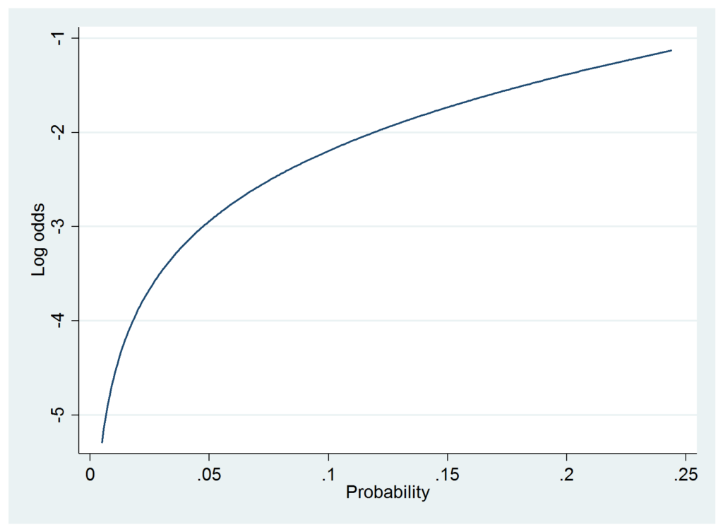
Clearly, there is substantial departure from linearity. But let’s go ahead and estimate the linear model anyway:
reg diabetes black female age, robust
I’ve requested robust standard errors to deal with any heteroskedasticity, but the t-statistics are about the same even without this option.
------------------------------------------------------------------------------
             |               Robust
    diabetes |      Coef.   Std. Err.      t    P>|t|     [95% Conf. Interval]
-------------+----------------------------------------------------------------
       black |   .0383148    .008328     4.60   0.000     .0219902    .0546393
      female |   .0068601   .0041382     1.66   0.097    -.0012515    .0149716
         age |   .0021575   .0001214    17.76   0.000     .0019194    .0023955
       _cons |  -.0619671   .0049469   -12.53   0.000    -.0716639   -.0522703
------------------------------------------------------------------------------
The t-statistics here are pretty close to the z-statistics for the logistic regression, and the coefficients themselves are quite similar to the AMEs shown above. But this model will not allow you to see how the effect of black on the probability of diabetes differs by age. For that, you’d have to explicitly build the interaction of those variables into the model, as I did in my previous post.
The upshot is that combining logistic regression with the margins command gives you the best of both worlds. You get a model that is likely to be a more accurate description of the world than a linear regression model. It will always produce predicted probabilities within the allowable range, and its parameters will tend to be more stable over varying conditions. On the other hand, you can also get numerical estimates that are interpretable as probabilities. And you can see how those probability-based estimates vary under different conditions.