
When using multiple imputation, you may wonder how many imputations you need. A simple answer is that more imputations are better. As you add more imputations, your estimates get more precise, meaning they have smaller standard errors (SEs). And your estimates get more replicable, meaning they would not change too much if you imputed the data again.
There are limits, though. No matter how many imputations you use, multiple imputation estimates can never be more precise or replicable than maximum likelihood estimates. And beyond a certain number of imputations, any improvement in precision and replicability becomes negligible.
So how many imputations are enough? An old rule of thumb was that 3 to 10 imputations typically suffice (Rubin 1987). But that advice only ensured the precision and replicability of point estimates. When the number of imputations is small, it is not uncommon to have point estimates that replicate well but SE estimates that do not.
LEARN MORE IN ONE OF OUR SHORT SEMINARS
In a recent paper (von Hippel 2018), for example, I estimated the mean body mass index (BMI) of first graders, from a sample where three quarters of BMI measurements were missing. With 5 imputations, the point estimate was 16.642 the first time I imputed the data, and 16.659 the second time. That’s good replicability; despite three quarters of the values being imputed, the two point estimates differed by just 0.1%.
But the SE estimate didn’t replicate as well; it was .023 the first time I imputed the data, and .026 the second time—a difference of 13%. Naturally, if the SE estimate isn’t replicable, related quantities like confidence intervals, t statistics, and p values won’t be replicable, either.
So you often need more imputations to get replicable SE estimates. But how many more? Read on.
A New Formula
I recently published a new formula (von Hippel 2018) that estimates how many imputations M you need for replicable SE estimates. The number of imputations is approximately
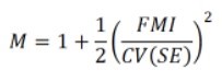
This formula depends on two quantities, FMI and CV(SE).
- FMI is the fraction of missing information. The FMI is not the fraction of values that are missing; it is the fraction by which the squared SE would shrink if the data were complete. You don’t need to figure out the FMI. Standard MI software gives you an estimate.
- CV() is a coefficient of variation, which you can think of as roughly the percentage by which you’d be willing to see the SE estimate change if the data were imputed again.
For example, if you have FMI=30 percent missing information, and you would accept the SE estimate changing by 10 percent if you imputed the data again, then you’ll only need M=5 or 6 imputations. But if you’d only accept the SE changing by 5%, then you’ll need M=19 imputations. (Naturally, the same formulas work if FMI and CV(SE) are expressed as proportions, .3 and .1, rather than percentages of 30 and 10.)
Notice that the number of imputations increases quadratically, with the square of FMI. This quadratic rule is better than an older rule M = 100 FMI, according to which the number of imputations should increase linearly with FMI (Bodner 2008; White et al. 2011).
Here’s a graph, adapted from von Hippel (2018), that fits the linear and quadratic rules to a simulation carried out by Bodner (2008), showing how many imputations are needed to achieve a goal similar to CV(SE)=.05. With that goal, the quadratic rule simplifies to M=1+200 FMI2, and the linear rule, as usual, is M=100 FMI.
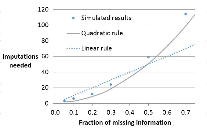
Clearly the quadratic rule fits the simulation better than the linear rule. The rules agree when FMI=0.5, but when FMI is larger, the linear rule underestimates the number of imputations needed, and when FMI is smaller, the linear rule overestimates the number of imputations needed. For example, with 20% missing information, the linear rule says that you need 20 imputations, but the quadratic rule says you can make do with 9.
When the fraction of missing information gets above 70%, both rules underestimate the number of imputations needed for stable t-based confidence intervals. I suspect that happens because the degrees of freedom in the t statistic becomes unstable (von Hippel 2018). I am looking at that issue separately.
A Two Step Recipe
A limitation of the quadratic rule is that FMI is not known in advance. FMI has to be estimated, typically by multiple imputation. And the estimate of FMI itself can be unreliable unless the number of imputations is large (Harel 2007).
So it’s a circular problem. You need an estimate of FMI to decide how many imputations you need. But you can’t get an estimate of FMI until you impute the data. For that reason, I recommend a two-step recipe (von Hippel, 2018):
- First, carry out a pilot analysis. Impute the data using a convenient number of imputations. (20 imputations is a reasonable default, if it doesn’t take too long.) Estimate the FMI by analyzing the imputed data.
- Next, plug the estimated FMI into the formula above to figure out how many imputations you need to achieve a certain value of CV(SE). If you need more imputations than you had in the pilot, then add those imputations and analyze the data again.
There are two small wrinkles:
First, when you plug an estimate of FMI into the formula, you shouldn’t use a point estimate. Instead, you should use the upper bound of a 95% confidence interval for FMI. That way you take only a 2.5% risk of having too few imputations in your final analysis.
Second, in your analysis you may estimate several parameters, as in a multiple regression. In that case, you have to decide which SEs you want to be replicable. If you don’t have a strong opinion, the simplest thing is to focus on the SE of the parameter with the largest FMI.
Software
The two-step recipe has been implemented in three popular data analysis packages.
- In Stata, you can install my command how_many_imputations by typing ssc install how_many_imputations.
- In SAS, you can use my macro %mi_combine, which is available in this Google Drive folder.
- In R, use Josh Errickson’s package howManyImputations, which is available through CRAN, here.
Alternatives
The two-stage procedure isn’t the only good way to find a suitable number of imputations. An alternative is to keep adding imputed datasets until the estimates converge, or change very little as new imputed datasets are added. This approach can be applied to any quantity you want to estimate—a point estimate, a standard error, a confidence interval, a p value. This approach, called iterative multiple imputation (Nassiri et al. 2018), has been implemented in the R package imi, which is available via GitHub, here.
Stata’s mi estimate command uses a jackknife procedure to estimate how much your standard error estimates and p values would change if the data were imputed again with the same number of imputations (Royston, Carlin, and White 2009). These jackknife estimates can give you some idea whether you need more imputations, but they can’t directly tell you how many imputations to add.
(An earlier, shorter version of this post appeared on missingdata.org in January 2018.)
Key reference
von Hippel, Paul T. (2020). “How many imputations do you need? A two-stage calculation using a quadratic rule.” Sociological Methods and Research, published online, behind a paywall. A free pre-publication version is available as an arXiv e-print.
See also
Bodner, T. E. (2008). What Improves with Increased Missing Data Imputations? Structural Equation Modeling, 15(4), 651–675. https://doi.org/10.1080/10705510802339072
Graham, J. W., Olchowski, A. E., & Gilreath, T. D. (2007). How Many Imputations are Really Needed? Some Practical Clarifications of Multiple Imputation Theory. Prevention Science, 8(3), 206–213. https://doi.org/10.1007/s11121-007-0070-9
Harel, O. (2007) Inferences on missing information under multiple imputation and two-stage multiple imputation. Statistical Methodology, 4(1), 75-89.
Nassiri, Vahid, Geert Molenberghs, Geert Verbeke, and João Barbosa-Breda. (2019). “Iterative Multiple Imputation: A Framework to Determine the Number of Imputed Datasets.” The American Statistician, 17 pages online ahead of print. https://doi.org/10.1080/00031305.2018.1543615
Royston, Patrick, John B. Carlin, and Ian R. White. (2009). “Multiple Imputation of Missing Values: New Features for Mim.” The Stata Journal 9(2):252–64.
Rubin, D. B. (1987). Multiple imputation for nonresponse in surveys. New York: Wiley.
White, I. R., Royston, P., & Wood, A. M. (2011). Multiple imputation using chained equations: Issues and guidance for practice. Statistics in Medicine, 30(4), 377–399. https://doi.org/10.1002/sim.4067
Comments
The instruction above for installing the Stata package causes an error:
. ssc install how_many_
ssc install: “how_many_” not found at SSC, type search how_many_
(To find all packages at SSC that start with h, type ssc describe h)
r(601);
You need to use the full command, as follows:
ssc install how_many_imputations
Cheers,
Bruce