
Seven years ago, I wrote a blog post about an alarming statistical problem discovered by Stephen Vaisey and Andrew Miles (hereafter V&M). In brief, they showed that if you estimate a linear, fixed effects model for panel data with lagged predictors, the results can be very misleading if the time lags are not correctly specified.
V&M (2017) investigated this problem for the case of three time periods, no lagged effect of the dependent variable y on itself, and no effect of y on the predictor x. They then posed the following question: Suppose that the true model is that y at time t depends only on x at the same time t, with a coefficient β. What happens if you unwittingly estimate a fixed effects model in which y depends only on x at time t-1?
Their answer is scary. Using both simulation and an algebraic proof, they showed that the expected value of the coefficient of x(t-1) is exactly -.5β. In other words, a positive contemporaneous effect of x gets transformed into an artifactually negative lagged effect.
In my 2015 post, I reported preliminary simulations indicating that the sign reversal can also happen
- with four or more time points.
- when the predictors of y include a lagged value of y.
- when y also has a lagged effect on x.
This might explain why some studies using fixed effects with lagged predictors (e.g., Ousey et al. 2011) have found negative lagged effects of x on y even though most previous research suggested positive effects. Unless there’s some solution to this problem, it would not be unreasonable to conclude that fixed effects with lagged predictors should never be used for causal inference. The one exception would be when you have total confidence that your data captures the correct lag structure—but how often does that happen?
LEARN MORE IN A SEMINAR WITH PAUL ALLISON
In that same 2015 post, I tentatively suggested a partial solution to the V&M problem: estimate a model in which y(t) is affected by both x(t)and x(t-1). Here’s what I said about interpreting the results:
If a one-year lag is the correct specification, then the contemporaneous effect should be small and not statistically significant. If, on the other hand, the contemporaneous effect is large and significant, it should raise serious doubts about the validity of the method and the kinds of conclusions that can be drawn. It may be that the data are simply not suitable for separating the effect of x on y from the effect of y on x.
This is essentially a robustness check. If the contemporaneous effect doesn’t show up, you’re good. If it does show up, all bets are off.
In a recent article, however, Leszczensky and Wolbring (2022) (hereafter L&W) argued that this is a complete solution. Just estimate a fixed effects model with both x(t) and x(t-1) as predictors of y(t), and you’re done! However, they also showed that not all fixed effects methods do a good job of this under more challenging conditions (such as a lagged effect of y on x). Based on simulations, they recommended the ML-SEM method developed by me and my colleagues, Richard Williams and Enrique Moral-Benito (2017). This method uses structural equation modeling software to estimate models that treat the fixed effects as latent random variables that are allowed to correlate with other exogenous variables. The method can also allow for “reverse causation” by including equations for effects of y on later values of x.
Although I’m happy that L&W settled on ML-SEM as the best available estimation method, I’m still not convinced that including a contemporaneous effect of x on y is the right way to go. One major objective of panel data analysis is to figure out whether x causes y or y causes x. If your model allows x to affect y at the same point in time, how do you know whether you’re estimating the effect of x on y or the effect of y on x? And if it’s really the latter, what impact will that have on the lagged effect of x?
In this post, I’m going to propose a better way. My proposal draws on a long tradition in the analysis of “cross-lagged panel models”, which is embodied in the path diagram below.
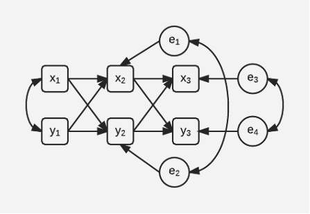
This diagram does not include fixed effects. But what it does include are correlations between the two error terms at each point in time (e1 with e2 and e3 with e4). These error terms capture the effects of unobserved variables that are affecting x and y at each point in time. The correlations between them are actually partial correlations that control for the earlier values of x and y. It makes perfect sense to include these partial correlations because otherwise the model would imply that any correlation between x(t) and y(t) is completely explained by their mutual dependence on x(t-1) and y(t-1). That seems highly implausible.
This model can be extended to included fixed effects using the ML-SEM method mentioned above. However, there are two things worth emphasizing:
- The models of V&M and the models of L&W implicitly set these error correlations to zero.
- If you allow these error correlations, the dreaded sign reversals discovered by V&M disappear, even without the inclusion of a contemporaneous effect of x on y or vice versa. I’ll provide evidence for that shortly.
So that’s it, that’s my idea—estimate models with lagged x using the ML-SEM method, but allow correlations between the error terms for x and y at each point in time.
That’s easy to do when you’re estimating a full-scale cross-lagged panel model like the one in the diagram above. But it’s not obvious how to do it when you’re estimating a “one-sided” model in which only y appears as a dependent variable, not x. In models like that, the ML-SEM method typically requires that x(t) be allowed to correlate with all earlier error variables, e.g., with e(t-1), e(t-2), e(t-3),…. This is equivalent to allowing x(t) to be affected by all earlier values of y. My proposal is to also let x(t) be correlated with e(t). That’s equivalent to allowing for a partial correlation between y(t) and x(t).
Again, that’s not hard to do if you’re coding the SEM model from scratch. But it is a problem for two user-written packages that are designed to simplify the ML-SEM method—xtdpdml for Stata and dpm for R. If you specify a predictor as “predetermined”, these two packages are set up to allow correlations between x(t) and all error terms prior to time t. To get the partial correlation model, it’s necessary to trick them into also allowing the correlation between x(t) and e(t). The trick is simple. You just create a lagged version of the x variable before entering it into the package commands. (I show how to do this for dpm in the appended simulation code.)
Now we have two competing methods for solving the V&M problem—the contemporaneous x solution and the partial correlation solution. To find out which is better, I replicated some of the simulations reported by L&W. Their equation for y(t) included x(t), x(t-1) and y(t-1) as predictors, with several different values for the coefficients.
Detailed results from my simulations are reported in the Appendix. The table below summarizes those results. “Conventional” refers to the use of ML-SEM with neither the contemporaneous effect of x nor the correlation of x(t) and e(t). A checkmark indicates that the method produced an unbiased estimate of the effect of x(t-1). An X indicates a biased estimate.
As expected, the conventional method estimates a lagged effect that is biased in all situations except one—when there is a true lagged effect and no contemporaneous effect.
| Model | True Model | Conventional | Contemporaneous x | Partial Correlation |
| 1 | x(t) affects y(t) x(t-1) doesn’t affect y(t) | X | ✔ | ✔ |
| 2 | x(t) doesn’t affect y( t) x(t-1) affects y(t) | ✔ | ✔ | ✔ |
| 3 | x(t) affects y(t) x(t-1) affects y(t) | X | ✔ | ✔ |
| 4 | y(t) affects x(t) x(t-1) affects y(t) | X | X | ✔ |
As L&W reported, the ML-SEM method with contemporaneous x does a good job of recovering the effect of x(t-1) on y(t) for Models 1-3. But so does ML-SEM with the partial correlation method.
Then I simulated data under Model 4, which was not considered by L&W. Instead of x(t) being affected by y(t-1), I let x(t) depend on y(t). I also deleted the effect of x(t) on y(t). The rationale for that change is that nothing in the data could help us decide whether y(t) affects x(t) or vice versa. So, we really need to try both possibilities to see what impact that has on the estimation methods. Results in the Appendix clearly show that the partial correlation method continues to do an excellent job of estimating the lagged effect of x, but the contemporaneous x method yields a biased estimate.
Is that the final word? Maybe, maybe not. As this example shows, the problem with simulation studies is that they can never cover all the possibilities. It’s quite possible that there are other plausible situations in which neither method does well. But for now, the partial correlation method seems like the better bet.
References
Allison, P. D., Williams, R., & Moral-Benito, E. (2017). Maximum likelihood for cross-lagged panel models with fixed effects. Socius, 3, https://doi.org/10.1177/2378023117710578
Leszczensky, L., & Wolbring, T. (2022). How to deal with reverse causality using panel data? Recommendations for researchers based on a simulation study. Sociological Methods & Research, 51(2), 837-865. https://doi.org/10.1177/0049124119882473
Ousey, G. C., Wilcox, P., & Fisher, B. S. (2011). Something old, something new: Revisiting competing hypotheses of the victimization-offending relationship among adolescents. Journal of Quantitative Criminology, 27(1), 53-84. https://doi.org/10.1007/s10940-010-9099-1
Vaisey, S., & Miles, A. (2017). What You Can—and Can’t—Do With Three-Wave Panel Data. Sociological Methods & Research, 46(1), 44–67. https://doi.org/10.1177/0049124114547769
Appendix
Here, I report simulations to compare the performance of the contemporaneous x method and the partial correlation method. I began with the model of L&W which says that
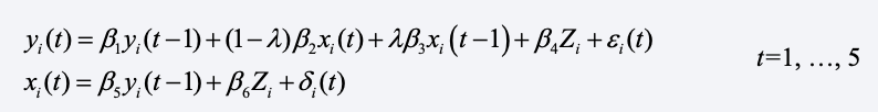
The disturbances, ei(t) and di(t), were simulated as independent standard normal variables. Similarly, xi(0) and yi(0) were simulated as standard normal variables with a correlation of .50. Time-invariant heterogeneity is represented by Zi which was standard normal, independent of xi(0), yi(0), and all ε’s and δ’s. The tuning parameter λ varies between 0 and 1, which shifts the model from an entirely contemporaneous effect of x to an entirely lagged effect. Note that the second equation allows for reverse causation, i.e., y affecting later values of x.
All programming was done in R (with code shown below). Because the goal was to investigate large sample bias, I generated a single sample of 10,000 cases for each set of parameter values. For each scenario, there were six time periods at which both x and y were observed. The variable Z was treated as unobserved.
Let’s begin with case of λ=0. In words, this says that there is a contemporaneous effect of x on y, but no lagged effect. This is the situation in which we would expect to find a sign reversal for a conventional fixed effects model that has only a lagged effect of x. Other parameters had the following values: β2 and β3 = 1, all other β’s = .5.
I estimated the one-sided equation for y using the dpm package in R. Here are the results.
| Predictor | True Value | Conventional | Contemp. x | Partial Corr. |
| x(t) | 1.0 | 0.993 | ||
| x(t-1) | 0.0 | -0.348 | -0.008 | -0.021 |
| y(t-1) | 0.5 | 1.068 | 0.503 | 1.012 |
The “conventional” column shows what you get when you lag x and y but use neither the contemporaneous x method or the partial correlation method. As V&M would predict, the “spurious” coefficient of lagged x is negative, although not exactly the -.5 value that they found in their much simpler model.
The “contemporaneous x” column shows that you get with the L&W method. All three coefficients are well estimated. Finally, the partial correlation method yields a good estimate of the lagged effect of x. Although it’s negative, it’s not significantly different from 0, even with a sample of 10,000 cases. On the other hand, the lagged effect of y is approximately double what it should be. That’s hardly ideal, although not a fatal flaw if the main goal is to estimate the effect of x on y. That result is also not surprising, given that we’ve excluded a key variable from the model.
The next step is to set λ = 1, which means that there is no contemporaneous effect of x but instead a lagged effect of x, specifically, β3 = 1. Here are the new results:
| Predictor | True Value | Conventional | Contemp. x | Partial Corr. |
| x(t) | 0.0 | -0.004 | ||
| x(t-1) | 1.0 | 0.999 | 0.998 | 0.997 |
| y(t-1) | 0.5 | 0.494 | 0.495 | 0.494 |
In this case, all three methods give approximately unbiased estimates for all three parameters.
For the last version of the L&W model, λ was set equal to 0.5 to give equal weight to contemporaneous and lagged effects of x. That produced the following results:
| Predictor | True Value | Conventional | Contemp. x | Partial Corr. |
| x(t) | 0.5 | 0.501 | ||
| x(t-1) | 0.5 | 0.357 | 0.504 | 0.502 |
| y(t-1) | 0.5 | 0.722 | 0.494 | 0.749 |
Not surprisingly, the results are midway between what we saw in the previous two scenarios. The conventional method underestimates the lagged effect of x and overestimates the lagged effect of y. The partial correlation method also overestimates the lagged effect of y, but gives the right answer for the lagged effect of x. The contemporaneous x method gets all three parameters correct.
At this point, we might conclude that both the contemporaneous x method and the partial correlation method do about equally well in estimating the lagged effect of x. However, we might prefer the contemporaneous x method because it also does a better job of estimating the lagged effect of y on itself when there is a true contemporaneous effect if x. Nevertheless, there are other scenarios that need to be considered.
In the next scenario, I modified the second equation in the L&W model by changing y(t-1) to y(t). Again, the rationale is that if we are willing to postulate a contemporaneous effect of x on y, we should also be willing to entertain a contemporaneous effect of y on x. Clearly, we cannot estimate a model that has both, so I set λ = 1 in the first equation, thereby eliminating x(t) from that equation.
Now the results show a clear superiority of the partial correlation method:
| Predictor | True Value | Conventional | Contemp. x | Partial Corr. |
| x(t) | 0.0 | 0.412 | ||
| x(t-1) | 1.0 | 0.849 | 0.807 | 1.005 |
| y(t-1) | 0.5 | 0.495 | 0.391 | 0.496 |
The contemporaneous x method is biased for all three coefficients. The conventional method is approximately unbiased for the lagged effect of y, but the lagged effect of x is biased downward. Only the partial correlation method gets all the coefficients right.
Finally, I also modified the equation for x(t) by adding x(t-1) as a predictor. It seemed to me that that if y had an autoregressive effect, x should also have one. Here are the results:
| Predictor | True Value | Conventional | Contemp. x | Partial Corr. |
| x(t) | 0.0 | 0.412 | ||
| x(t-1) | 1.0 | 0.837 | 0.601 | 1.008 |
| y(t-1) | 0.5 | 0.578 | 0.387 | 0.493 |
Once again, the partial correlation method gets it right. And the bias for the contemporaneous x has gotten substantially worse.
If your primary interest is in the lagged effect of x on y, the partial correlation method seems like the way to go. Unlike the contemporaneous x method, it is approximately unbiased under all scenarios considered. Nevertheless, there are many more possible variations to be explored. So, this evidence should only be considered preliminary.
R Code for Simulations
library(panelr)
library(dpm)
library(dplyr)

set.seed(6781)
n <- 10000
b1 <- .5
b2 <- 1
b3 <- 1
b4 <- .5
b5 <- .5
b6 <- .5

#### Data Generation: Contemporaneous Effect of x on y, no lagged effect.
L <- 0
z <- rnorm(n)
x_0 <- rnorm(n)
y_0 <- .5*x_0 + sqrt(1-.5^2)*rnorm(n)
x_1 <- b5*y_0 + b6*z + rnorm(n)
y_1 <- b1*y_0 + (1-L)*b2*x_1 + L*b3*x_0 + b4*z + rnorm(n)
x_2 <- b5*y_1 + b6*z + rnorm(n)
y_2 <- b1*y_1 + (1-L)*b2*x_2 + L*b3*x_1 + b4*z + rnorm(n)
x_3 <- b5*y_2 + b6*z + rnorm(n)
y_3 <- b1*y_2 + (1-L)*b2*x_3 + L*b3*x_2 + b4*z + rnorm(n)
x_4 <- b5*y_3 + b6*z + rnorm(n)
y_4 <- b1*y_3 + (1-L)*b2*x_4 + L*b3*x_3 + b4*z + rnorm(n)
x_5 <- b5*y_4 + b6*z + rnorm(n)
y_5 <- b1*y_4 + (1-L)*b2*x_5 + L*b3*x_4 + b4*z + rnorm(n)
dat <- data.frame(z,x_0,y_0,x_1,y_1,x_2,y_2,x_3,y_3,x_4,y_4,x_5,y_5)
dat.long<-long_panel(dat, periods=c(0:5), prefix="_",
                       label_location = "end")
#Estimation: only lag x
out <- dpm(y ~ pre(lag(x)), data=dat.long, error.inv=T)
summary(out)

#Estimation: x + lag x
out <- dpm(y ~ pre(x) + pre(lag(x)), data=dat.long, error.inv=T)
summary(out)

#Estimation: lag x with partial correlation
dat.lag <- dat.long %>%
  group_by(id) %>%
  mutate(lag1_x = lag(x, n=1, order_by=id))
out <- dpm(y ~ pre(lag1_x), data=dat.lag, error.inv=T)
summary(out)

####Data Generation:  A lagged effect of x on y, no contemporaneous effect.
set.seed(5324)
L <- 1
z <- rnorm(n)
x_0 <- rnorm(n)
y_0 <- .5*x_0 + sqrt(1-.5^2)*rnorm(n)
x_1 <- b5*y_0 + b6*z + rnorm(n)
y_1 <- b1*y_0 + (1-L)*b2*x_1 + L*b3*x_0 + b4*z + rnorm(n)
x_2 <- b5*y_1 + b6*z + rnorm(n)
y_2 <- b1*y_1 + (1-L)*b2*x_2 + L*b3*x_1 + b4*z + rnorm(n)
x_3 <- b5*y_2 + b6*z + rnorm(n)
y_3 <- b1*y_2 + (1-L)*b2*x_3 + L*b3*x_2 + b4*z + rnorm(n)
x_4 <- b5*y_3 + b6*z + rnorm(n)
y_4 <- b1*y_3 + (1-L)*b2*x_4 + L*b3*x_3 + b4*z + rnorm(n)
x_5 <- b5*y_4 + b6*z + rnorm(n)
y_5 <- b1*y_4 + (1-L)*b2*x_5 + L*b3*x_4 + b4*z + rnorm(n)
dat <- data.frame(z,x_0,y_0,x_1,y_1,x_2,y_2,x_3,y_3,x_4,y_4,x_5,y_5)
dat.long<-long_panel(dat, periods=c(0:5), prefix="_",
                     label_location = "end")
#Estimation: only lag x
out <- dpm(y ~ pre(lag(x)), data=dat.long, error.inv=T)
summary(out)

#Estimation:  x + lag x
out <- dpm(y ~ pre(x) + pre(lag(x)), data=dat.long, error.inv=T)
summary(out)

#Estimation: lag x with partial correlation
dat.lag <- dat.long %>%
  group_by(id) %>%
  mutate(lag1_x = lag(x, n=1, order_by=id))
out <- dpm(y ~ pre(lag1_x), data=dat.lag, error.inv=T)
summary(out)

####Data Generation:   Equal lagged and contemporaneous effects of x. set.seed(66657)
L <- .5
z <- rnorm(n)
x_0 <- rnorm(n)
y_0 <- .5*x_0 + sqrt(1-.5^2)*rnorm(n)
x_1 <- b5*y_0 + b6*z + rnorm(n)
y_1 <- b1*y_0 + (1-L)*b2*x_1 + L*b3*x_0 + b4*z + rnorm(n)
x_2 <- b5*y_1 + b6*z + rnorm(n)
y_2 <- b1*y_1 + (1-L)*b2*x_2 + L*b3*x_1 + b4*z + rnorm(n)
x_3 <- b5*y_2 + b6*z + rnorm(n)
y_3 <- b1*y_2 + (1-L)*b2*x_3 + L*b3*x_2 + b4*z + rnorm(n)
x_4 <- b5*y_3 + b6*z + rnorm(n)
y_4 <- b1*y_3 + (1-L)*b2*x_4 + L*b3*x_3 + b4*z + rnorm(n)
x_5 <- b5*y_4 + b6*z + rnorm(n)
y_5 <- b1*y_4 + (1-L)*b2*x_5 + L*b3*x_4 + b4*z + rnorm(n)
dat <- data.frame(z,x_0,y_0,x_1,y_1,x_2,y_2,x_3,y_3,x_4,y_4,x_5,y_5)
dat.long<-long_panel(dat, periods=c(0:5), prefix="_",
                     label_location = "end")
#Estimation: only lag x
out <- dpm(y ~ pre(lag(x)), data=dat.long, error.inv=T)
summary(out)

#Estimation:  x + lag x
out <- dpm(y ~ pre(x) + pre(lag(x)), data=dat.long, error.inv=T)
summary(out)

#Estimation: lag x with partial correlation
dat.lag <- dat.long %>%
  group_by(id) %>%
  mutate(lag1_x = lag(x, n=1, order_by=id))
out <- dpm(y ~ pre(lag1_x), data=dat.lag, error.inv=T)
summary(out)


#####Data Generation: x affected by contemporaneous y   ############
library(panelr)
library(dpm)
set.seed(6708)
n <- 10000
b1 <- .5 #effect of y(t-1) on y(t)
b3 <- 1 #effect of x(t-1) on y(t)
b4 <- .5 #effect of z on y
b5 <- .5 #effect of y(t) on x(t)
b6 <- .5 #effect of z on x
z <- rnorm(n)
x_0 <- rnorm(n)
y_0 <- .5*x_0 + sqrt(1-.5^2)*rnorm(n)
y_1 <- b1*y_0 + b3*x_0 + b4*z + rnorm(n)
x_1 <- b5*y_1 + b6*z + rnorm(n)
y_2 <- b1*y_1 + b3*x_1 + b4*z + rnorm(n)
x_2 <- b5*y_2 + b6*z + rnorm(n)
y_3 <- b1*y_2 + b3*x_2 + b4*z + rnorm(n)
x_3 <- b5*y_3 + b6*z + rnorm(n)
y_4 <- b1*y_3 + b3*x_3 + b4*z + rnorm(n)
x_4 <- b5*y_4 + b6*z + rnorm(n)
y_5 <- b1*y_4 + b3*x_4 + b4*z + rnorm(n)
x_5 <- b5*y_5 + b6*z + rnorm(n)

dat <- data.frame(z,x_0,y_0,x_1,y_1,x_2,y_2,x_3,y_3,x_4,y_4,x_5,y_5)
dat.long<-long_panel(dat, periods=c(0:5), prefix="_",
                     label_location = "end")

#Estimation: only lag x
out <- dpm(y ~ pre(lag(x)), data=dat.long, error.inv=T)
summary(out)

#Estimation: x + lag x
out <- dpm(y ~ pre(x) + pre(lag(x)), data=dat.long, error.inv=T)
summary(out)

#Estimation: lag x with partial correlation
dat.lag <- dat.long %>%
  group_by(id) %>%
  mutate(lag1_x = lag(x, n=1, order_by=id))
out <- dpm(y ~ pre(lag1_x), data=dat.lag, error.inv=T)
summary(out)

#####Data Generation:   x affected by contemporaneous y + lagged x   ############
library(panelr)
library(dpm)
set.seed(6708)
n <- 10000
b1 <- .5 #effect of y(t-1) on y(t)
b2 <- 1 #effect of x(t) on y(t)
b3 <- 1 #effect of x(t-1) on y(t)
b4 <- .5 #effect of z on y
b5 <- .5 #effect of y(t) on x(t)
b6 <- .5 #effect of z on x
L <- 1
z <- rnorm(n)
x_0 <- rnorm(n)
y_0 <- .5*x_0 + sqrt(1-.5^2)*rnorm(n)
y_1 <- b1*y_0 + b3*x_0 + b4*z + rnorm(n)
x_1 <- b5*y_1 + .5*x_0 + b6*z + rnorm(n)
y_2 <- b1*y_1 + b3*x_1 + b4*z + rnorm(n)
x_2 <- b5*y_2 + .5*x_1 + b6*z + rnorm(n)
y_3 <- b1*y_2 + b3*x_2 + b4*z + rnorm(n)
x_3 <- b5*y_3 + .5*x_2 + b6*z + rnorm(n)
y_4 <- b1*y_3 + b3*x_3 + b4*z + rnorm(n)
x_4 <- b5*y_4 + .5*x_3 + b6*z + rnorm(n)
y_5 <- b1*y_4 + b3*x_4 + b4*z + rnorm(n)
x_5 <- b5*y_5 + .5*x_4 + b6*z + rnorm(n)

dat <- data.frame(z,x_0,y_0,x_1,y_1,x_2,y_2,x_3,y_3,x_4,y_4,x_5,y_5)
dat.long<-long_panel(dat, periods=c(0:5), prefix="_",
                     label_location = "end")

#Estimation: only lag x
out <- dpm(y ~ pre(lag(x)), data=dat.long, error.inv=T)
summary(out)

#Estimation: x + lag x
out <- dpm(y ~ pre(x) + pre(lag(x)), data=dat.long, error.inv=T)
summary(out)

#Estimation: lag x with partial correlation
dat.lag <- dat.long %>%
  group_by(id) %>%
  mutate(lag1_x = lag(x, n=1, order_by=id))
out <- dpm(y ~ pre(lag1_x), data=dat.lag, error.inv=T)
summary(out)
Comments
I am looking at an economic paper to be found here:
https://www.researchgate.net/publication/334625793_Determinants_of_the_profit_rates_in_the_OECD_economies_-_a_panel_data_analysis_of_the_Kaleckian_profit_equation
In that paper the author uses panel data to evaluate the extent to which the identity associated with Kalecki in the text is confirmed by the evidence.
Briefly, Kalecki proposed that there is an identity associating trade balance (exports-imports), government deficit or surplus and investment v consumption with six variables.
He discusses causal relationships between the variables, within the time period of observation. Kalecki mentioned in his writings that there was a lag applicable in at least one case.
One purpose that the author had was to determine causal aspects between the variables, the other was to verify the identity itself. It seems to me that it is not possible to do both. What to do for each?
Sorry but I don’t have an answer.