Instrumental Variables in Structural Equation Models

When I teach courses on structural equation modeling (SEM), I tell my students that any model with instrumental variables can be estimated in the SEM framework. Then I present a classic example of simultaneous causation in which X affects Y, and Y also affects X. Models like this can be estimated if each of the two variables also has an instrumental variable—a variable that affects it but not the other variable. Specification of the model is fairly straightforward in any SEM package.

However, there are lots of other uses of instrumental variables. My claim that they can all be estimated with SEM is more speculative than I usually care to admit. A couple weeks ago I got a question about instrumental variables in SEM that really had me stumped. What seemed like the right way to do it was giving the wrong answer—at least not the answer produced by all the standard econometric methods, like two-stage least squares (2SLS) or the generalized method of moments (GMM). When I finally hit on the solution, I figured that others might benefit from what I had learned. Hence, this blog post.

LEARN MORE IN A SEMINAR WITH PAUL ALLISON

The question came from Steven Utke, an assistant professor of accounting at the University of Connecticut. Steve was trying to replicate a famous study by David Card (1995) that attempted to estimate the causal effect of education on wages by using proximity to college as an instrumental variable. Steve was able to replicate Card’s 2SLS analysis, but he couldn’t get an SEM model to produce similar results.

For didactic purposes, I’m going to greatly simplify Card’s analysis by excluding a lot of variables that are not essential for the example. I’ll use Stata for the analysis, but equivalent SAS code can be found in Addendum 2.

Let’s begin with a bivariate regression of the log of hourly wages on years of education, for a sample of 3,010 young men in 1976.

. use "https://dl.dropboxusercontent.com/s/bu8ze4db4bywwin/card", clear
. gen lwage = log(wage)
. regress lwage educ

------------------------------------------------------------------------------
       lwage |      Coef.   Std. Err.      t    P>|t|     [95% Conf. Interval]
-------------+----------------------------------------------------------------
        educ |   .0520942   .0028697    18.15   0.000     .0464674     .057721
       _cons |   5.570882   .0388295   143.47   0.000     5.494747    5.647017
------------------------------------------------------------------------------

Education has a highly significant coefficient, whose magnitude can be interpreted as follows: each additional year of schooling is associated with about a 5% increase in wages.

Of course, the problem with treating this as a causal effect is that there are likely to be many omitted variables that affect both education and wages. We could control for those variables by measuring them and including them in the model (and Card did that for many variables). But there’s no way we can control for all the possible confounding variables, especially because some variables are difficult to measure (e.g., ability). We must therefore conclude that education is correlated with the error term in the regression (a form of endogeneity), and that our regression coefficient is therefore biased to an unknown degree.

Card proposed to solve this problem by introducing proximity to college as an instrumental variable. Specifically, nearc4 was a dummy (indicator) variable for whether or not the person was raised in a local labor market that included a four-year college. As with any instrumental variable, the crucial assumption was that nearc4 would affect years of schooling but would NOT directly affect lwage. Although there may be reasons to doubt that assumption (some discussed by Card), they are not relevant to our discussion here.

Using the ivregress command in Stata, I estimated the instrumental variable model by 2SLS. In case you’re not familiar with that venerable method, it amounts to this: (a) do an OLS regression of educ on nearc4, (b) calculate predicted values from that regression, and (c) regress lwage on those predicted values. The only tricky part is getting the standard errors right. Here are the results:

. ivregress 2sls lwage (educ=nearc4)

Instrumental variables (2SLS)
------------------------------------------------------------------------------
       lwage |      Coef.   Std. Err.      z    P>|z|     [95% Conf. Interval]
-------------+----------------------------------------------------------------
        educ |   .1880626   .0262826     7.16   0.000     .1365497    .2395756
       _cons |   3.767472   .3487458    10.80   0.000     3.083942    4.451001
------------------------------------------------------------------------------

Instrumented:  educ
Instruments:   nearc4

Remarkably, the coefficient for education in this regression is more than three times as large as in the bivariate regression and is still highly significant. According to this estimate, each additional year of schooling yields a 21% increase in wages (calculated as 100(exp(.188)-1), a very large effect by any reasonable standard.  (Card got a coefficient of around .14 with other predictors in the model).

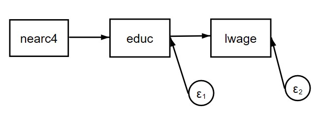
Now let’s try to do this with a structural equation model, using Stata’s sem command. As with all SEM software, the default is to do maximum likelihood estimation under the assumption of multivariate normality. The basic idea is to specify a model in which nearc4 affects educ, and educ affects lwage.  But there can be no direct effect of nearc4 on lwage.  Here’s a path diagram for the model:

Here’s the Stata code and the results:

. sem (lwage <- educ) (educ <- nearc4)

------------------------------------------------------------------------------
             |      Coef.   Std. Err.      z    P>|z|     [95% Conf. Interval]
-------------+----------------------------------------------------------------
Structural   |
  lwage      |
        educ |   .0520942   .0028688    18.16   0.000     .0464716    .0577169
       _cons |   5.570882   .0388166   143.52   0.000     5.494803    5.646961
  -----------+----------------------------------------------------------------
  educ       |
      nearc4 |    .829019   .1036643     8.00   0.000     .6258406    1.032197
       _cons |   12.69801   .0856132   148.32   0.000     12.53022    12.86581

This can’t be right, however, because the coefficient for educ is identical to what we got in our initial bivariate regression, with an almost identical standard error. Clearly, the inclusion of the regression of educ on nearc4 has accomplished nothing. Can this problem be fixed, and if so, how?

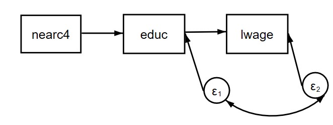
I struggled with this for about an hour before it hit me. The solution is to build into the model the very thing that we are trying to correct for with the instrumental variable. If there are omitted variables that are affecting both educ and lwage, they should produce a correlation between the error term for educ and the error term for lwage. That correlation needs to be included in the SEM model. Here’s a path diagram for the new model:

In Stata, it’s done like this:

. sem (lwage <-educ) (educ<-nearc4), cov(e.educ*e.lwage)

The cov option allows a covariance (and therefore a correlation) between the two error terms. Here are the new results:

------------------------------------------------------------------------------------
                   |      Coef.   Std. Err.      z    P>|z|     [95% Conf. Interval]
-------------------+----------------------------------------------------------------
Structural         |
  lwage            |
              educ |   .1880626   .0262826     7.16   0.000     .1365497    .2395756
             _cons |   3.767472   .3487458    10.80   0.000     3.083942    4.451001
  -----------------+----------------------------------------------------------------
  educ             |
            nearc4 |    .829019   .1036643     8.00   0.000     .6258406    1.032197
             _cons |   12.69801   .0856132   148.32   0.000     12.53022    12.86581
-------------------+----------------------------------------------------------------

Now the coefficient and standard error for educ are identical to what we saw earlier with 2SLS. Problem solved! (SEM won’t always give identical results to 2SLS, as I explain in Addendum 1).

Interestingly, the estimated correlation between the error terms (not shown in the table) was -.66. That means that the collective impact of omitted variables is to affect educ and lwage in opposite directions. Whatever raises lwage lowers educ, and vice versa.

It’s hard to imagine what variables would behave like this. And that difficulty raises questions about the plausibility of the model. (Card suggested that measurement error in education could produce a negative correlation, but the degree of error would have to be unreasonably large to produce the result we just saw.) In any case, that’s not really our concern here. It does point out, however, that one of the advantages of the SEM approach is that you get an estimate of the error correlation—something you typically don’t see with 2SLS.

What’s the lesson here?  If you want to use SEM to estimate an instrumental variable model, it’s essential to think carefully about why you need instruments in the first place. You should make sure that the specified model reflects all your beliefs about the causal mechanism. In particular, if you suspect that error terms are correlated with observed variables, those correlations must be built into the model.

If you’d like to learn more about structural equation modeling, check out my on-demand SEM courses: Part 1 for beginners, and Part 2 for those who already have some knowledge of SEM. You might also be interested in Felix Elwert’s course on Instrumental Variables.

Reference:

Card, David (1995) “Using geographic variation in college proximity to estimate the return to schooling.” Aspects of Labour Economics: Essays in Honour of John Vanderkamp. University of Toronto Press.

Addendum 1.  Just-Identified Models

The reason 2SLS and SEM produce identical coefficient estimates for this example is that the model is just-identified. That is, the model imposes no restrictions on the variances and covariances of the variables. Other instrumental variable methods like limited information maximum likelihood or GMM also yield identical results in the just-identified situation. For models that are over-identified (for example, if there are two instrumental variables instead of just one), these methods will all yield somewhat different results.

Addendum 2.  SAS code

Go to http://davidcard.berkeley.edu/data_sets.html to get the data set as a text file along with a sas program for reading in the data.  Here is the code for the analysis:

proc reg data=card;
  model lwage76 = ed76;
proc syslin 2sls data=card;
  endogenous ed76;
  instruments nearc4;
  model lwage76 = ed76;
proc calis data=card;
  path
    lwage76 <- ed76,
    ed76 <- nearc4;
proc calis data=card;
  path
    lwage76 <- ed76,
    ed76 <- nearc4,
    ed76 <-> lwage76; *This specifies a correlation between the error terms;
run;